🔨 Text as data in R

Session 09

10.01.2024

print("Hello course!")

👨‍💻 Christoph Adrian

Schedule

Session Datum Topic Presenter

Introduction

1

25.10.2023

Kick-Off

Christoph Adrian

01.11.2023

🎃 Holiday (No Lecture)

2

08.11.2023

Einführung in DBD

Christoph Adrian

3

15.11.2023

🔨 Working with R

Christoph Adrian

🗣️

Presentations

4

22.11.2023

📚 Media routines & habits

Group C

5

29.11.2023

~📚 Digital disconnection~

6

06.12.2023

📚 Digital disconnection

Group A

7

13.12.2023

📦 Data collection methods

Group D

8

20.12.2023

📦 Automatic text analysis 🎥

Group B

🎄Christmas Break (No Lecture)

📂 Project

Analysis of media content

9

10.01.2024

🔨 Text as data

Christoph Adrian

10

17.01.2024

🔨 Automatic analysis of text in R

Christoph Adrian

11

24.01.2024

🔨 Q&A

Christoph Adrian

12

31.01.2024

📊 Presentation & Discussion

All groups

13

07.02.2024

🏁 Recap, Evaluation & Discussion

Christoph Adrian

Agenda

  1. Digital disconnection on
  2. Text as data in R (Part I)
  3. 📋 Hands on working with R

Digital disconnection on (not 𝕏)

Background on the research project & data

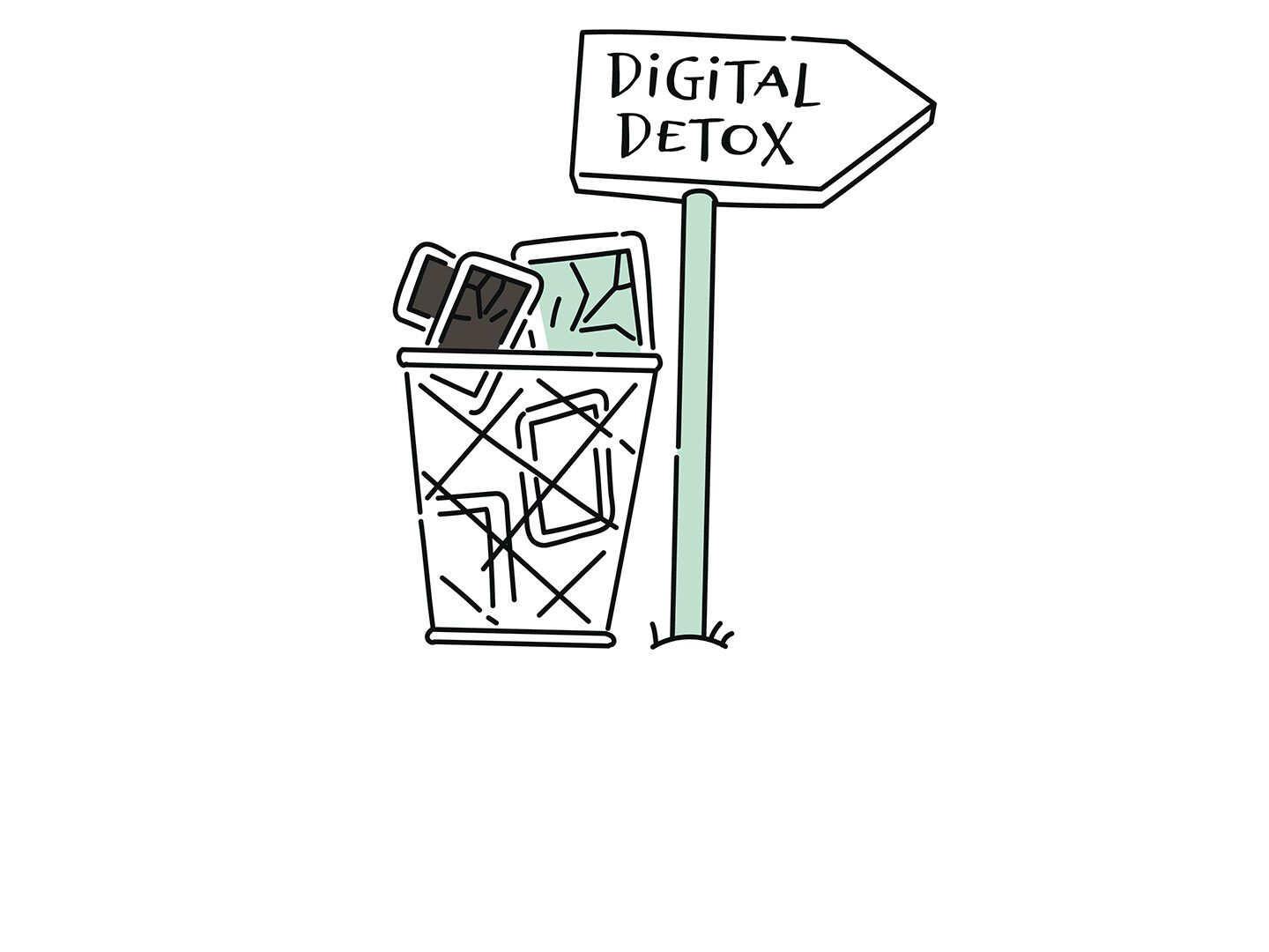
Looking at the discourse

The theoretical background: digital disconnection

  • Increasing trend towards more conscious use of digital media (devices), including (deliberate) non-use with the aim to restore or improve psychological well-being (among other factors)

  • But how do “we” talk (on Twitter) about digital detox/disconnection:
    Is social media a 💊 drug, 👹 demon or 🍩 donut?


Source: dup-magazin.de

Social Media as 💊, 👹 or 🍩 ?

Relationship between social media use, digital well-being and digital disconnection

Social Media as a …
Drug Demon Donut

What is at stake?

Addiction/health

Distraction

Well-being

Root cause of problem

Individual susceptibility

Addictive design

Inadequate fit

User agency

Agency is limited due to innate susceptibilities

Agency needs to be reclaimed from social media platforms

User has agency, but it is challenged by person-, technology- and context-specific elements

Focus of disconnection

Complete abstinence, re-training of the ‘faulty brain’ to break the dopamine link

Removing/weakening the distracting potential of tech, using persuasive design to support exerting social media self-control

Disconnection interventions tailored to persons and/or contexts to ‘optimize the balance’ between benefits and drawbacks of connectivity, mindful use

Digital disconnection examples

Digital detox, cognitive behavioral therapy

Muting phone, disabling notifications, putting phone in grey-scale, using apps that reward abstinence (e.g., Forest)

Locative disconnection, disconnection apps that extensive tailoring to persons and contexts, mindfulness training

(Vanden Abeele et al., 2022)

digital detox, #digitaldetox, …

Information about the data collection process

  • Goal: Collect all tweets (until 31.12.2022) that mention or discuss digital detox (and similar terms) on Twitter (not 𝕏)
  • Actual collection was done in the beginning of 2023 (before the takeover by Musk and the associated change in API access)
  • Access via Twitter Academic Research Product Track v2 API with the help of the academictwitteR package (Barrie & Ho, 2021)
academictwitteR::build_query(
  query = c("digital detox", "#digitaldetox", "digital_detox"),
  is_retweet = FALSE
  )

A quick glimpse

The structure of the data set & available variables

tweets_correct %>% glimpse()
Rows: 361,408
Columns: 37
$ tweet_id               <chr> "7223508762", "7222271007", "7219735500", "7216…
$ user_username          <chr> "Princessbride24", "winnerandy", "the_enthusias…
$ text                   <chr> "@Ali_Sweeney detox same week as the digital cl…
$ created_at             <dttm> 2009-12-31 05:25:55, 2009-12-31 04:44:20, 2009…
$ in_reply_to_user_id    <chr> "23018333", NA, NA, NA, NA, NA, NA, "19475829",…
$ author_id              <chr> "16157429", "14969949", "16217478", "18001568",…
$ lang                   <chr> "en", "en", "en", "en", "en", "en", "en", "en",…
$ possibly_sensitive     <lgl> FALSE, FALSE, FALSE, FALSE, FALSE, FALSE, FALSE…
$ conversation_id        <chr> "7222577237", "7222271007", "7219735500", "7216…
$ user_created_at        <chr> "2008-09-06T15:13:58.000Z", "2008-06-01T07:34:3…
$ user_protected         <lgl> FALSE, FALSE, FALSE, FALSE, FALSE, FALSE, FALSE…
$ user_name              <chr> "Sam", "Andrew", "The Enthusiast", "🌻BahSun🌻"…
$ user_verified          <lgl> FALSE, FALSE, FALSE, FALSE, FALSE, FALSE, FALSE…
$ user_description       <chr> "As you wish.", "Life is a playground, so enjoy…
$ user_location          <chr> "Houston", "California", "Melbourne, Australia"…
$ user_url               <chr> "https://t.co/hchLJvesW1", NA, "http://t.co/bLK…
$ user_profile_image_url <chr> "https://pbs.twimg.com/profile_images/587051289…
$ user_pinned_tweet_id   <chr> NA, NA, NA, NA, "1285575168010735621", NA, NA, …
$ retweet_count          <int> 0, 0, 0, 0, 0, 0, 0, 0, 0, 0, 0, 0, 0, 0, 0, 0,…
$ like_count             <int> 0, 0, 1, 0, 0, 0, 0, 0, 0, 0, 0, 0, 0, 0, 0, 0,…
$ quote_count            <int> 0, 0, 0, 0, 0, 0, 0, 0, 0, 0, 0, 0, 0, 0, 0, 0,…
$ user_tweet_count       <int> 3905, 18808, 4494, 35337, 284181, 18907, 39562,…
$ user_list_count        <int> 7, 12, 101, 49, 540, 82, 91, 12, 117, 46, 192, …
$ user_followers_count   <int> 103, 481, 2118, 693, 17677, 2527, 8784, 100, 26…
$ user_following_count   <int> 370, 1488, 391, 317, 16470, 320, 11538, 120, 25…
$ sourcetweet_type       <chr> NA, NA, NA, NA, NA, NA, NA, NA, NA, NA, NA, NA,…
$ sourcetweet_id         <chr> NA, NA, NA, NA, NA, NA, NA, NA, NA, NA, NA, NA,…
$ sourcetweet_text       <chr> NA, NA, NA, NA, NA, NA, NA, NA, NA, NA, NA, NA,…
$ sourcetweet_lang       <chr> NA, NA, NA, NA, NA, NA, NA, NA, NA, NA, NA, NA,…
$ sourcetweet_author_id  <chr> NA, NA, NA, NA, NA, NA, NA, NA, NA, NA, NA, NA,…
$ year                   <dbl> 2009, 2009, 2009, 2009, 2009, 2009, 2009, 2009,…
$ month                  <dbl> 12, 12, 12, 12, 12, 12, 12, 12, 12, 12, 12, 12,…
$ day                    <int> 31, 31, 31, 31, 30, 30, 30, 29, 28, 28, 27, 27,…
$ hour                   <int> 5, 4, 3, 1, 22, 2, 0, 20, 21, 1, 19, 8, 8, 3, 9…
$ minute                 <int> 25, 44, 22, 42, 49, 31, 39, 23, 45, 47, 31, 28,…
$ retweet_dy             <lgl> FALSE, FALSE, FALSE, FALSE, TRUE, FALSE, FALSE,…
$ detox_dy               <lgl> FALSE, FALSE, FALSE, FALSE, FALSE, FALSE, FALSE…

Biggest attention in 2016, steady decline thereafter

Distribution of tweets with reference to digital detox over time

Expand for full code
tweets_correct %>% 
  ggplot(aes(x = as.factor(year), fill = retweet_dy)) +
    geom_bar() +
    labs(
      x = "",
      y = "Number of tweets", 
      fill = "Is the tweet a retweet?"
     ) +
    scale_fill_manual(values = c("#1DA1F2", "#004389")) +
    theme_pubr() +    
    # add annotations
    annotate(
      "text", 
      x = 14, y = 55000,
      label = "Increase of character limit from 140 to 280") + 
    geom_curve(
      data = data.frame(
        x = 14.2965001234837,y = 53507.2283841571,
        xend = 11.5275706534335, yend = 45412.4966032138),
      mapping = aes(x = x, y = y, xend = xend, yend = yend),
      angle = 127L,
      curvature = 0.28,
      arrow = arrow(30L, unit(0.1, "inches"), "last", "closed"),
      inherit.aes = FALSE)

Sporadic tweeting on the topic, mainly in English

Tweets with reference to ditigal detox by (participating) users and language

# Number of tweets by user 
tweets_correct %>% 
    group_by(author_id) %>% 
    summarize(n = n()) %>% 
    mutate(
        n_grp = case_when(
                     n <=    1 ~ 1,
            n >   1 & n <=  10 ~ 2,
            n >  10 & n <=  25 ~ 3,
            n >  25 & n <=  50 ~ 4,
            n >  50 & n <=  75 ~ 5,
            n >  75 & n <= 100 ~ 6,
            n > 100 ~ 7
        ), 
        n_grp_fct = factor(
            n_grp,
            levels = c(1:7),
            labels = c(
            " 1",
            " 2 - 10", "11 - 25",
            "26 - 50", "50 - 75",
            "75 -100", "> 100")
        )
    ) %>% 
    sjmisc::frq(n_grp_fct) %>% 
    as.data.frame() %>% 
    select(val, frq:cum.prc) %>% 
    # create table
    gt() %>% 
    # tab_header(
    #     title = "Tweets by users with a least on tweet"
    #    ) %>% 
    cols_label(
      val = "Number of tweets by user",
      frq = "n",
      raw.prc = html("%<sub>raw</sub>"),
      cum.prc = html("%<sub>cum</sub>")
  ) %>% 
  gt_theme_538()
# Language of Tweets
tweets_correct %>% 
    sjmisc::frq(
        lang, 
        sort.frq = c("desc"), 
        min.frq = 2000
    ) %>% 
    as.data.frame() %>% 
    select(val, frq:cum.prc) %>% 
    # create table
    gt() %>% 
    # tab_header(
    #     title = "Language of the collected tweets"
    #   ) %>% 
    cols_label(
      val = "Twitter language code",
      frq = "n",
      raw.prc = html("%<sub>raw</sub>"),
      cum.prc = html("%<sub>cum</sub>")
  ) %>% 
  gt_theme_538()
Expand for full code
Number of tweets by user n %raw %cum
1 143364 77.21 77.21
2 - 10 39981 21.53 98.74
11 - 25 1647 0.89 99.63
26 - 50 435 0.23 99.86
50 - 75 88 0.05 99.91
75 -100 55 0.03 99.94
> 100 109 0.06 100.00
NA 0 0.00 NA
Expand for full code
Twitter language code n %raw %cum
en 274351 75.91 75.91
fr 20407 5.65 81.56
es 16248 4.50 86.05
de 14091 3.90 89.95
pt 7127 1.97 91.92
it 5999 1.66 93.58
da 3490 0.97 94.55
in 3095 0.86 95.41
ja 2428 0.67 96.08
n < 2000 14172 3.92 100.00
NA 0 0.00 NA

Text as data in R

Part I: Basics of tidy text wrangling & sentiment analysis

Deciding on the right method

Different approaches of computational analysis of text

  • No method that is the one, but specific applications for specific methods

  • Apart from analyzing basic word and text metrics, there are three variants of automatic text analysis:

    • 🔎 Dictionary Approaches (e.g. Sentiment Analysis)

    • Unsupervised Text Analysis (e.g. Topic Modeling)

    • Supervised Text Analysis (e.g. ML Classifier)

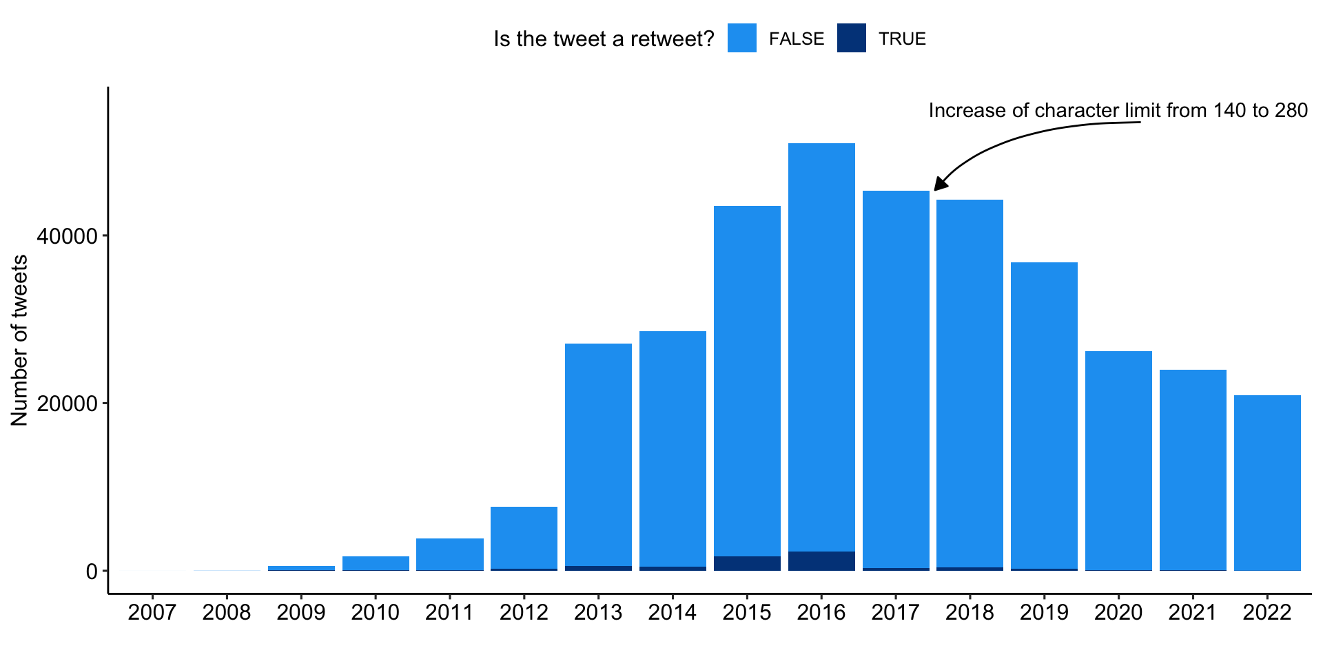
Building a shared vocabulary

Important terms & definitions

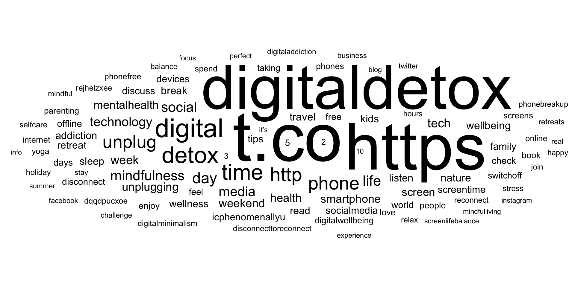
Explore tweets with #digitaldetox

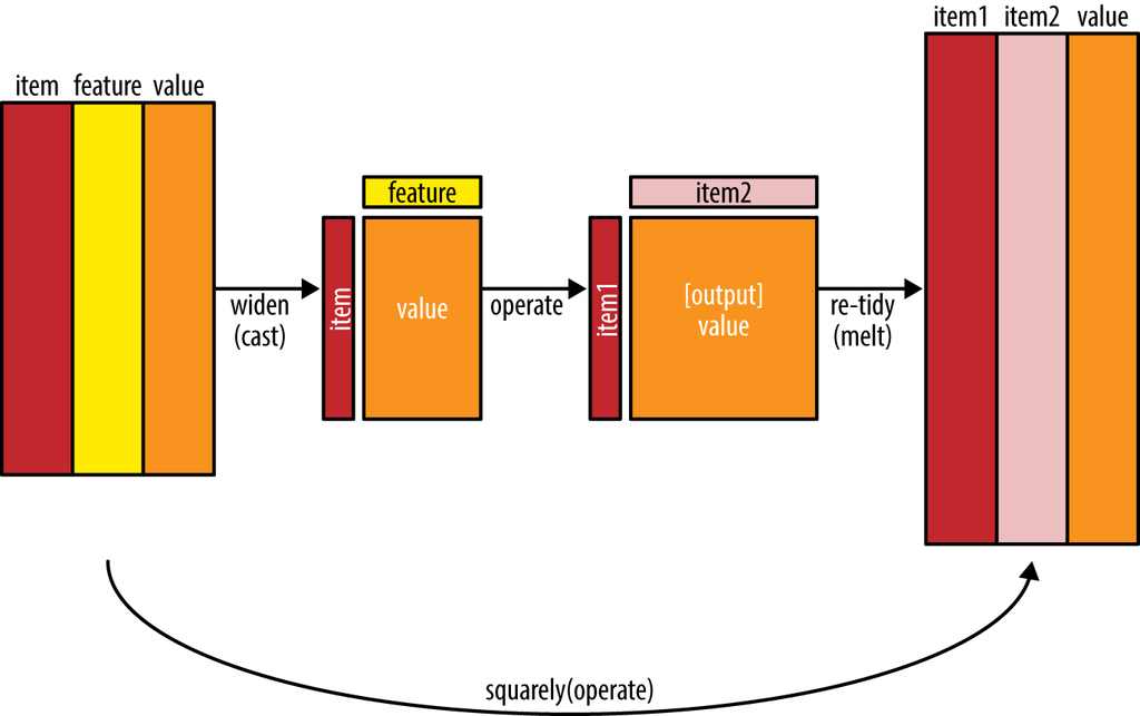
Working through a typical text analysis using tidy data principles

Test

(Silge & Robinson, 2017)

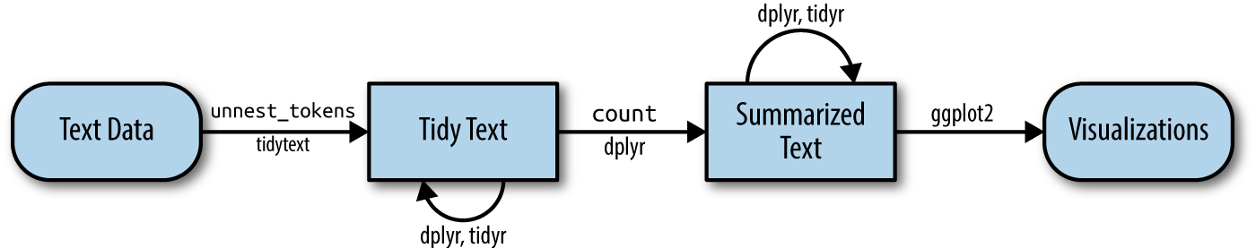
  • But: Tidy data has a specific structure:
    • Each variable is a column
    • Each observation is a row
    • Each type of observational unit is a table.
  • Thus the tidy text format is defined as a table with one-token-per-row (Silge & Robinson, 2017).

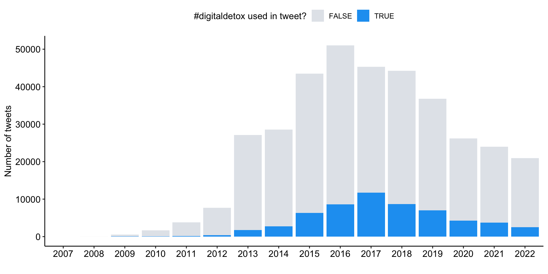
Focusing on #digitaldetox

Build a subsample

tweets_detox <- tweets_correct %>% 
  filter(
    detox_dy == TRUE, # only tweets with #digitaldetox
    retweet_dy == FALSE, # no retweets
    lang == "en" # only english tweets
    )
Expand for full code
tweets_correct %>% 
  ggplot(aes(x = as.factor(year), fill = detox_dy)) +
    geom_bar() +
    labs(
      x = "",
      y = "Number of tweets", 
      fill = "#digitaldetox used in tweet?"
     ) +
    scale_fill_manual(values = c("#A0ACBD50", "#1DA1F2")) +
    theme_pubr() 

Tokenization of the tweets

Transform data to tidy text

# Common HTML entities
remove_reg <- "&amp;|&lt;|&gt;"

# Create tidy data
tweets_tidy <- tweets_detox %>% 
    # Remove HTML entities
    mutate(text = str_remove_all(text, remove_reg)) %>% 
    # Tokenization
    tidytext::unnest_tokens("text", text) %>% 
    # Remove stopwords
    filter(!text %in% tidytext::stop_words$word)

# Preview
tweets_tidy %>% 
    select(tweet_id, user_username, text) %>% 
    print(n = 5)
# A tibble: 639,459 × 3
  tweet_id   user_username text      
  <chr>      <chr>         <chr>     
1 5777201122 pblackshaw    blackberry
2 5777201122 pblackshaw    iphone    
3 5777201122 pblackshaw    read      
4 5777201122 pblackshaw    pew       
5 5777201122 pblackshaw    report    
# ℹ 639,454 more rows

Count token frequency

Summarize all tokens over all tweets

# Create summarized data
tweets_summarized <- tweets_tidy %>% 
  count(text, sort = TRUE) 

# Preview Top 15 token
tweets_summarized %>% 
    print(n = 15)
# A tibble: 87,172 × 2
   text             n
   <chr>        <int>
 1 t.co         57530
 2 https        52890
 3 digitaldetox 46642
 4 digital       8521
 5 detox         6623
 6 time          6000
 7 http          4674
 8 phone         4213
 9 unplug        4021
10 day           2939
11 life          2548
12 social        2449
13 mindfulness   2408
14 media         2264
15 technology    2065
# ℹ 87,157 more rows

The (Unavoidable) Word Cloud

Visualization of Top 100 token

tweets_summarized %>% 
    top_n(100) %>% 
    ggplot(aes(label = text, size = n)) +
    ggwordcloud::geom_text_wordcloud() +
    scale_size_area(max_size = 30) +
    theme_minimal()

More than just single words

Modeling realtionships between words: n-grams and correlations

Many interesting text analyses are based on the relationships between words

  • whether examining which words tend to follow others immediately (n-grams),
  • or that tend to co-occur within the same documents (correlation)

Combinations of words

Count word pairs within tweets

# Create word paris
tweets_word_pairs <- tweets_tidy %>% 
    widyr::pairwise_count(
        text,
        tweet_id,
        sort = TRUE)

# Preview
tweets_word_pairs %>% 
    print(n = 15)
# A tibble: 3,466,216 × 3
   item1        item2            n
   <chr>        <chr>        <dbl>
 1 t.co         digitaldetox 40640
 2 digitaldetox t.co         40640
 3 t.co         https        36605
 4 https        t.co         36605
 5 https        digitaldetox 36486
 6 digitaldetox https        36486
 7 digital      digitaldetox  7791
 8 digitaldetox digital       7791
 9 t.co         digital       7365
10 digital      t.co          7365
11 https        digital       6856
12 digital      https         6856
13 detox        digitaldetox  6004
14 digitaldetox detox         6004
15 t.co         detox         5672
# ℹ 3,466,201 more rows

Correlation of words

Summarize and correlate tokens within tweets

# Create word correlation
tweets_pairs_corr <- tweets_tidy %>% 
    group_by(text) %>% 
    filter(n() >= 300) %>% 
    pairwise_cor(
        text, 
        tweet_id, 
        sort = TRUE)

# Preview
tweets_pairs_corr %>% 
    print(n = 15)
# A tibble: 41,820 × 3
   item1           item2           correlation
   <chr>           <chr>                 <dbl>
 1 jocelyn         brewer                0.999
 2 brewer          jocelyn               0.999
 3 jocelyn         discusses             0.983
 4 discusses       jocelyn               0.983
 5 discusses       brewer                0.982
 6 brewer          discusses             0.982
 7 icphenomenallyu discuss               0.981
 8 discuss         icphenomenallyu       0.981
 9 taniamulry      wealth                0.979
10 wealth          taniamulry            0.979
11 jocelyn         nutrition             0.968
12 nutrition       jocelyn               0.968
13 nutrition       brewer                0.967
14 brewer          nutrition             0.967
15 discusses       nutrition             0.951
# ℹ 41,805 more rows

Correlates of detox and digital

Display correlates for specific token

tweets_pairs_corr %>% 
  filter(
    item1 %in% c("detox", "digital")
    ) %>% 
  group_by(item1) %>% 
  slice_max(correlation, n = 5) %>% 
  ungroup() %>% 
  mutate(
    item2 = reorder(item2, correlation)
    ) %>% 
  ggplot(
    aes(item2, correlation, fill = item1)
    ) +
  geom_bar(stat = "identity") +
  facet_wrap(~ item1, scales = "free") +
  coord_flip() +
  scale_fill_manual(
    values = c("#C50F3C", "#04316A")) +
  theme_pubr()

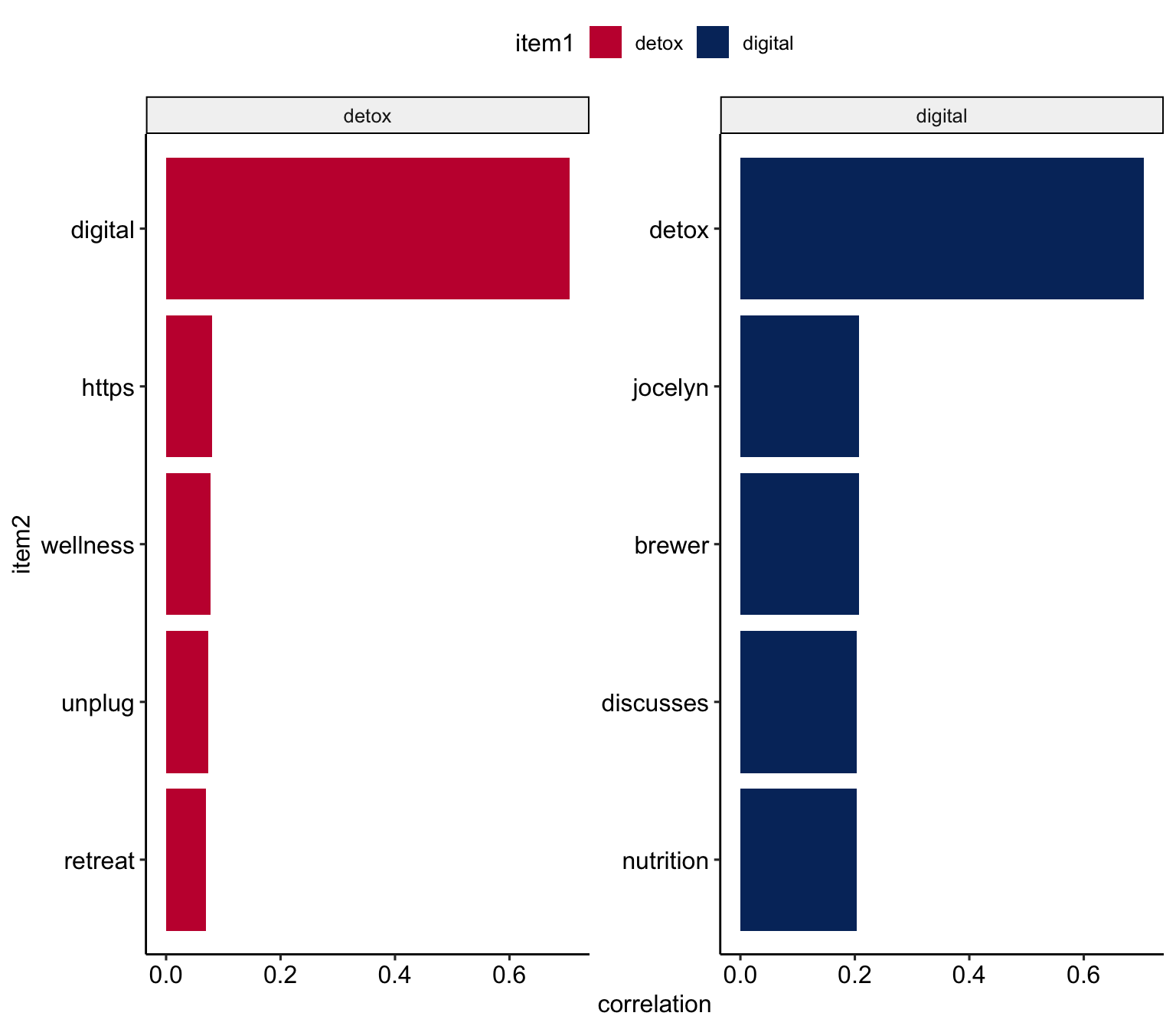
Let’s talk about sentiments

Dictionary based approach of text analysis

(Silge & Robinson, 2017)

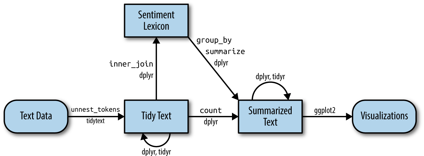
Atteveldt et al. (2021) argue that sentiment, in fact, are quite a complex concepts that are often hard to capture with dictionaries.

The meaning of “positive/negative”

Most commmon positive and negative words

tweets_sentiment_count <- tweets_tidy %>% 
  inner_join(
     get_sentiments("bing"),
     by = c("text" = "word"),
     relationship = "many-to-many") %>% 
  count(text, sentiment)
  
# Preview
tweets_sentiment_count %>% 
  group_by(sentiment) %>%
  slice_max(n, n = 10) %>% 
  ungroup() %>% 
  mutate(text = reorder(text, n)) %>%
  ggplot(aes(n, text, fill = sentiment)) +
  geom_col(show.legend = FALSE) +
  facet_wrap(
    ~sentiment, scales = "free_y") +
  labs(x = "Contribution to sentiment",
       y = NULL) +
  scale_fill_manual(
    values = c("#C50F3C", "#007D29")) +
  theme_pubr()

Enrich the original data

tweets_sentiment <- tweets_tidy %>% 
  inner_join(
     get_sentiments("bing"),
     by = c("text" = "word"),
     relationship = "many-to-many") %>% 
  count(tweet_id, sentiment) %>% 
  pivot_wider(names_from = sentiment, values_from = n, values_fill = 0) %>% 
  mutate(sentiment = positive - negative)
  
# Check
tweets_sentiment 
# A tibble: 24,372 × 4
   tweet_id            positive negative sentiment
   <chr>                  <int>    <int>     <int>
 1 1000009901563838465        3        0         3
 2 1000038819520008193        1        0         1
 3 1000042717492187136        4        0         4
 4 1000043574673715203        1        1         0
 5 1000075155891281925        4        0         4
 6 1000086637987139590        1        0         1
 7 1000094334660825088        1        0         1
 8 1000133715194920960        1        0         1
 9 1000255467434729472        0        1        -1
10 1000271209353895938        1        1         0
# ℹ 24,362 more rows

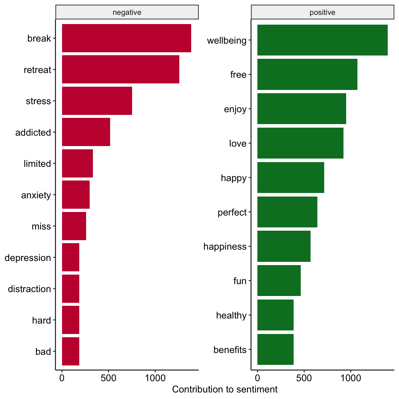
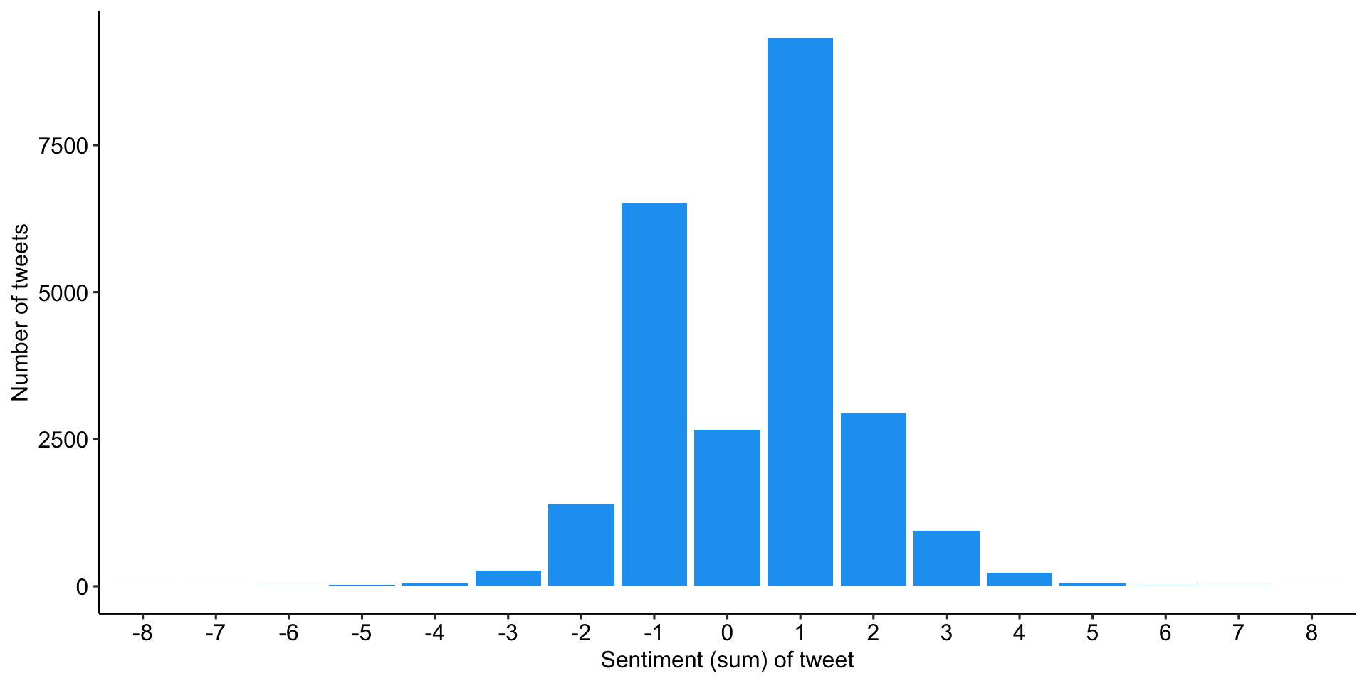
Slightly more positive tweets than negative

Overall distribution sentiment by tweets

tweets_sentiment %>% 
  ggplot(aes(as.factor(sentiment))) +
  geom_bar(fill = "#1DA1F2") +
  labs(
    x = "Sentiment (sum) of tweet", 
    y = "Number of tweets"
  ) +
  theme_pubr()

A trend towards positivity?

Development of tweet sentiment over the years

Expand for full code
# Create first graph
g1 <- tweets_correct %>% 
  filter(tweet_id %in% tweets_sentiment$tweet_id) %>% 
  left_join(tweets_sentiment) %>% 
  sjmisc::rec(
    sentiment,
    rec = "-8:-1=negative; 0=neutral; 1:8=positive") %>%
  ggplot(aes(x = as.factor(year), fill = as.factor(sentiment_r))) +
    geom_bar() +
    labs(
      x = "",
      y = "Number of tweets", 
      fill = "Sentiment (sum) of tweet") +
    scale_fill_manual(values = c("#C50F3C", "#90A0AF", "#007D29")) +
    theme_pubr() 
    #theme(axis.text.x = element_text(angle = 90, vjust = 0.5, hjust=1))

# Create second graph
g2 <- tweets_correct %>% 
  filter(tweet_id %in% tweets_sentiment$tweet_id) %>% 
  left_join(tweets_sentiment) %>% 
  sjmisc::rec(
    sentiment,
    rec = "-8:-1=negative; 0=neutral; 1:8=positive") %>%
  ggplot(aes(x = as.factor(year), fill = as.factor(sentiment_r))) +
    geom_bar(position = "fill") +
    labs(
      x = "",
      y = "Proportion of tweets", 
      fill = "Sentiment (sum) of tweet") +
    scale_fill_manual(values = c("#C50F3C", "#90A0AF", "#007D29")) +
    theme_pubr() 

# COMBINE GRPAHS
ggarrange(g1, g2,
          nrow = 1, ncol = 2, 
          align = "hv",
          common.legend = TRUE) 
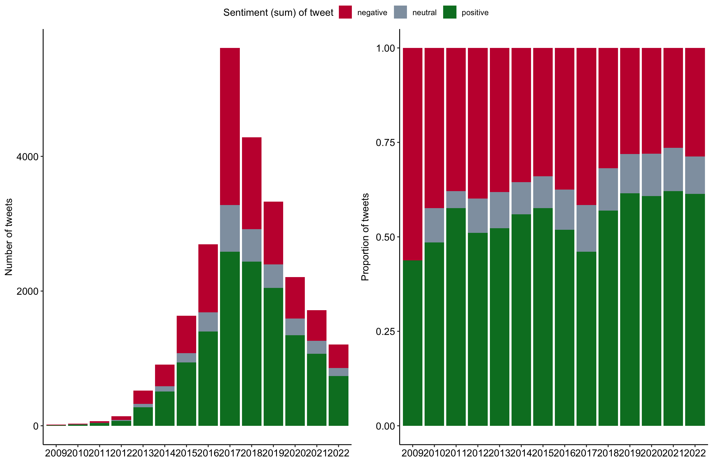
📋 Hands on working with R

Various exercises on the content of today’s session

🧪 And now … you: Clean and repeat!

Redo the tidy text analysis pipeline with cleaned data

Objective of this exercise

  • Brush up basic knowledge of working with R and the tidyverse
  • Get to know the typical steps of tidy text analysis, from tokenisation and summarisation to visualisation.

Next steps

  • Download files provided on StudOn or shared drives for the sessions
  • Unzip the archive at a destination of your choice.
  • Double click on the Exercise-Text_as_data.Rproj to open the RStudio project. This ensures that all dependencies are working correctly.
  • Open the exercise.qmd file and follow the instructions.
  • Tip: You can find all code chunks used in the slides in the showcase.qmd (for the raw code) or showcase.html (with rendered outputs).

Time for questions

Thank you and see you next week!

References

Atteveldt, W. van, Trilling, D., & Arcíla, C. (2021). Computational analysis of communication: A practical introduction to the analysis of texts, networks, and images with code examples in python and r. John Wiley & Sons.
Barrie, C., & Ho, J. (2021). academictwitteR: An r package to access the twitter academic research product track v2 API endpoint. Journal of Open Source Software, 6(62), 3272. https://doi.org/10.21105/joss.03272
Silge, J., & Robinson, D. (2017). Text mining with r: A tidy approach (First edition). O’Reilly.
Vanden Abeele, M. M. P., Halfmann, A., & Lee, E. W. J. (2022). Drug, demon, or donut? Theorizing the relationship between social media use, digital well-being and digital disconnection. Current Opinion in Psychology, 45, 101295. https://doi.org/10.1016/j.copsyc.2021.12.007