🔨 Automatic text analysis in R

Session 10

17.01.2024

`print("Hello (again)!")`

👨‍💻 Christoph Adrian

PhD student @ Chair of Communication Science
Text as Data & Social Media Usage (Effects)
Conversational in R, Beginner in Python, SPSS & Stata

Schedule

Session	Datum	Topic	Presenter
		Introduction
1	25.10.2023	Kick-Off	Christoph Adrian
	01.11.2023	🎃 Holiday (No Lecture)
2	08.11.2023	Einführung in DBD	Christoph Adrian
3	15.11.2023	🔨 Working with R	Christoph Adrian
	🗣️	Presentations
4	22.11.2023	📚 Media routines & habits	Group C
₅	29.11.2023	~📚 Digital disconnection~
6	06.12.2023	📚 Digital disconnection	Group A
7	13.12.2023	📦 Data collection methods	Group D
8	_20.12.2023	📦 Automatic text analysis 🎥	Group B
		🎄Christmas Break (No Lecture)
	📂 Project	Analysis of media content
9	10.01.2024	🔨 Text as data	Christoph Adrian
10	17.01.2024	🔨 Automatic analysis of text in R	Christoph Adrian
11	24.01.2024	🔨 Q&A	Christoph Adrian
12	31.01.2024	📊 Presentation & Discussion	All groups
13	07.02.2024	🏁 Recap, Evaluation & Discussion	Christoph Adrian

Agenda

What we did so far
Text as data in R (Part II)
📋 Hands on working with R

What we did so far

Analysis of tweets about digital disconnection on (not 𝕏)

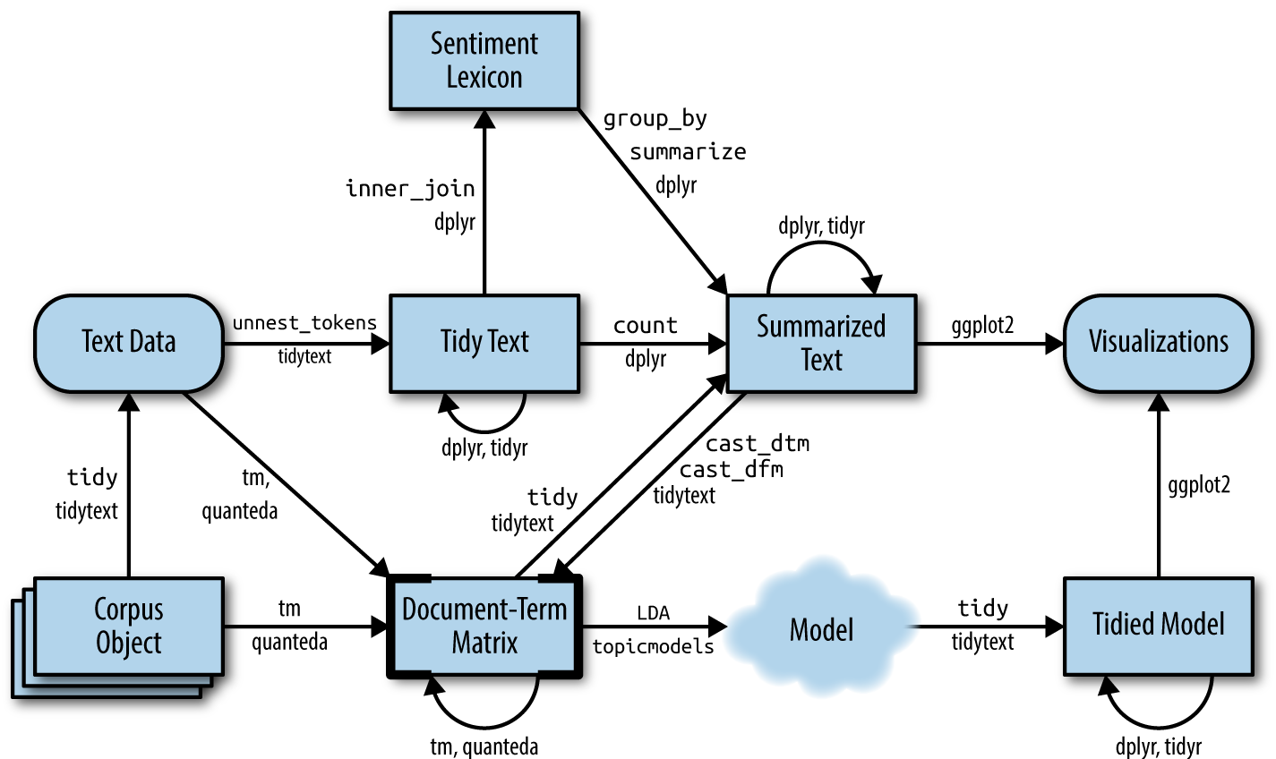
The tidy text format pipeline basics

Focus on single words and their relationship documents & sentiments

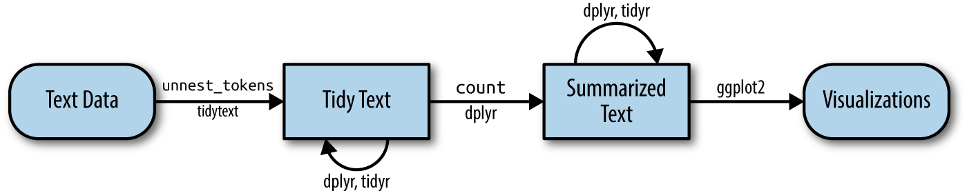
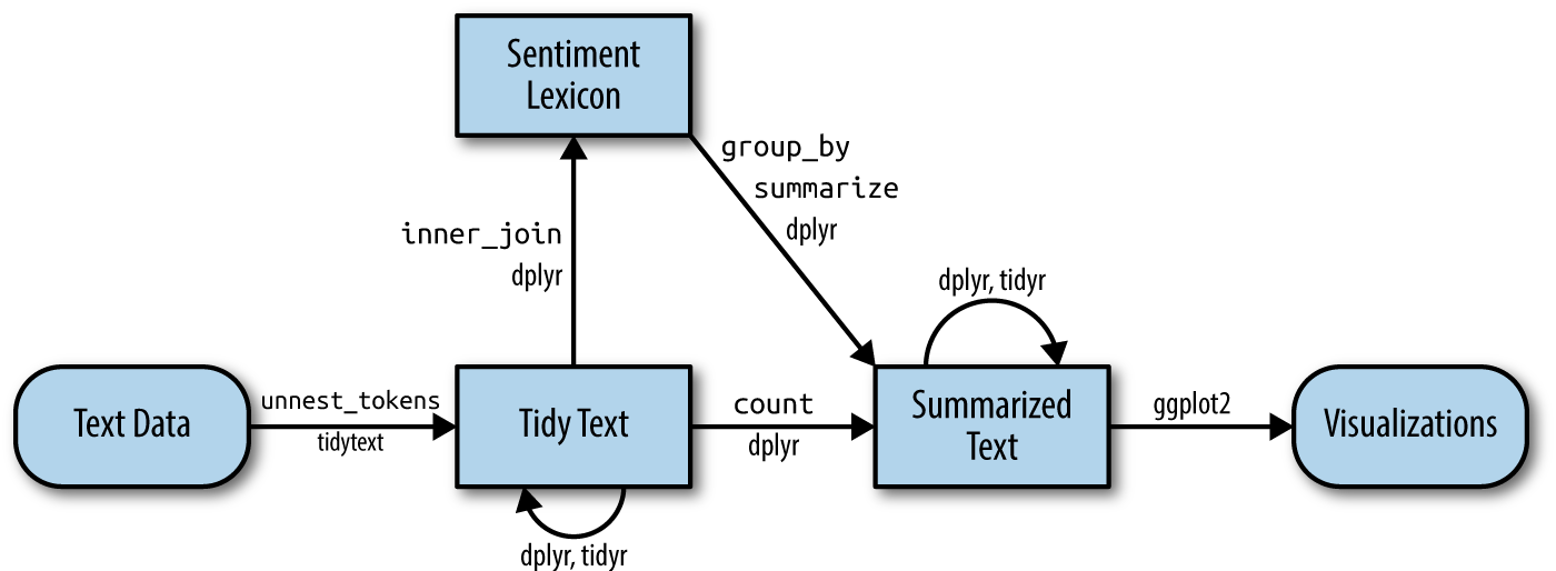
Silge & Robinson (2017)

Text as data in R

Part II: Document-Term-Matrices & Unsupervised Text Analysis (Topic Modeling)

Expansion of the pipeline

Focus on modeling the realtionships between words & documents

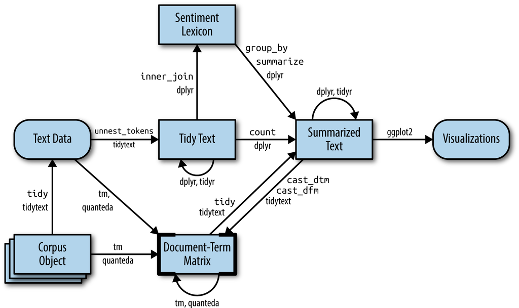
Silge & Robinson (2017)

Quick recap on Document-Term Matrix [DTM]

Most common structure for (classic) text mining

A matrix where:

each row represents one document (such as a tweet),
each column represents one term, and
each value (typically) contains the number of appearances of that term in that document.

(Zheng & Casari, 2018)

Step-by-step DTM creation

Along the tidy text pipeline: Tokenize

# Common HTML entities
remove_reg <- "&amp;|&lt;|&gt;"

# Create tidy data
tweets_tidy <- tweets_detox %>% 
  mutate(
    text = str_remove_all(text, remove_reg)) %>% 
    tidytext::unnest_tokens("text", text) %>% 
    filter(!text %in% tidytext::stop_words$word)

# Preview
tweets_tidy %>% 
  select(tweet_id, user_name, text) %>% 
  print(n = 15)

# A tibble: 639,459 × 3
   tweet_id   user_name      text        
   <chr>      <chr>          <chr>       
 1 5777201122 Pete Blackshaw blackberry  
 2 5777201122 Pete Blackshaw iphone      
 3 5777201122 Pete Blackshaw read        
 4 5777201122 Pete Blackshaw pew         
 5 5777201122 Pete Blackshaw report      
 6 5777201122 Pete Blackshaw teens       
 7 5777201122 Pete Blackshaw distracted  
 8 5777201122 Pete Blackshaw driving     
 9 5777201122 Pete Blackshaw http        
10 5777201122 Pete Blackshaw bit.ly      
11 5777201122 Pete Blackshaw 4abr5p      
12 5777201122 Pete Blackshaw digitaldetox
13 4814687834 Andrew Gerrard dawn_wylie  
14 4814687834 Andrew Gerrard prompted    
15 4814687834 Andrew Gerrard question    
# ℹ 639,444 more rows

Step-by-step DTM creation

Along the tidy text pipeline: Tokenize ▶️ Summarize

# Common HTML entities
remove_reg <- "&amp;|&lt;|&gt;"

# Create tidy data
tweets_tidy <- tweets_detox %>% 
  mutate(
    text = str_remove_all(text, remove_reg)) %>% 
    tidytext::unnest_tokens("text", text) %>% 
    filter(!text %in% tidytext::stop_words$word)

# Create summarized data
tweets_summarized <- tweets_tidy %>% 
  count(tweet_id, text) 

# Preview 
tweets_summarized %>% 
  print(n = 15)

# A tibble: 592,499 × 3
   tweet_id            text              n
   <chr>               <chr>         <int>
 1 1000009901563838465 bite              1
 2 1000009901563838465 detox             1
 3 1000009901563838465 digital           1
 4 1000009901563838465 digitaldetox      1
 5 1000009901563838465 enjoy             2
 6 1000009901563838465 fly               1
 7 1000009901563838465 happitizer        1
 8 1000009901563838465 happitizers       1
 9 1000009901563838465 https             1
10 1000009901563838465 inspiration       1
11 1000009901563838465 mindgourmet       1
12 1000009901563838465 mindgourmet’s     1
13 1000009901563838465 sized             1
14 1000009901563838465 t.co              1
15 1000009901563838465 taste             1
# ℹ 592,484 more rows

Step-by-step DTM creation

Along the tidy text pipeline: Tokenize ▶️ Summarize ▶️ DTM

# Common HTML entities
remove_reg <- "&amp;|&lt;|&gt;"

# Create tidy data
tweets_tidy <- tweets_detox %>% 
  mutate(
    text = str_remove_all(text, remove_reg)) %>% 
    tidytext::unnest_tokens("text", text) %>% 
    filter(!text %in% tidytext::stop_words$word)

# Create summarized data
tweets_summarized <- tweets_tidy %>% 
  count(tweet_id, text) 

# Create DTM
tweets_dtm <- tweets_summarized %>% 
  cast_dtm(tweet_id, text, n)

# Preview
tweets_dtm

<<DocumentTermMatrix (documents: 46670, terms: 87172)>>
Non-/sparse entries: 592499/4067724741
Sparsity           : 100%
Maximal term length: 49
Weighting          : term frequency (tf)

Choose or combine styles

Simple with tidytext, precise with quanteda

# Common HTML entities
remove_reg <- "&amp;|&lt;|&gt;"

# Create tidy data
tweets_tidy <- tweets_detox %>% 
  mutate(
    text = str_remove_all(text, remove_reg)) %>% 
    tidytext::unnest_tokens("text", text) %>% 
    filter(!text %in% tidytext::stop_words$word)

# Create summarized data
tweets_summarized <- tweets_tidy %>% 
  count(tweet_id, text) 

# Create DTM
tweets_dtm <- tweets_summarized %>% 
  cast_dtm(tweet_id, text, n)

# Preview
tweets_dtm

# Create corpus
quanteda_corpus <- tweets_detox %>% 
  quanteda::corpus(
    docid_field = "tweet_id", 
    text_field = "text"
  )

# Tokenize
quanteda_token <- quanteda_corpus %>% 
  quanteda::tokens(
    remove_punct = TRUE,
    remove_symbols = TRUE, 
    remove_numbers = TRUE, 
    remove_url = TRUE, 
    split_tags = FALSE # keep hashtags and mentions
  ) %>% 
  quanteda::tokens_tolower() %>% 
  quanteda::tokens_remove(
    pattern = stopwords("en")
    )

# Convert to Document-Feature-Matrix (DFM)
quanteda_dfm <- quanteda_token %>% 
  quanteda::dfm()

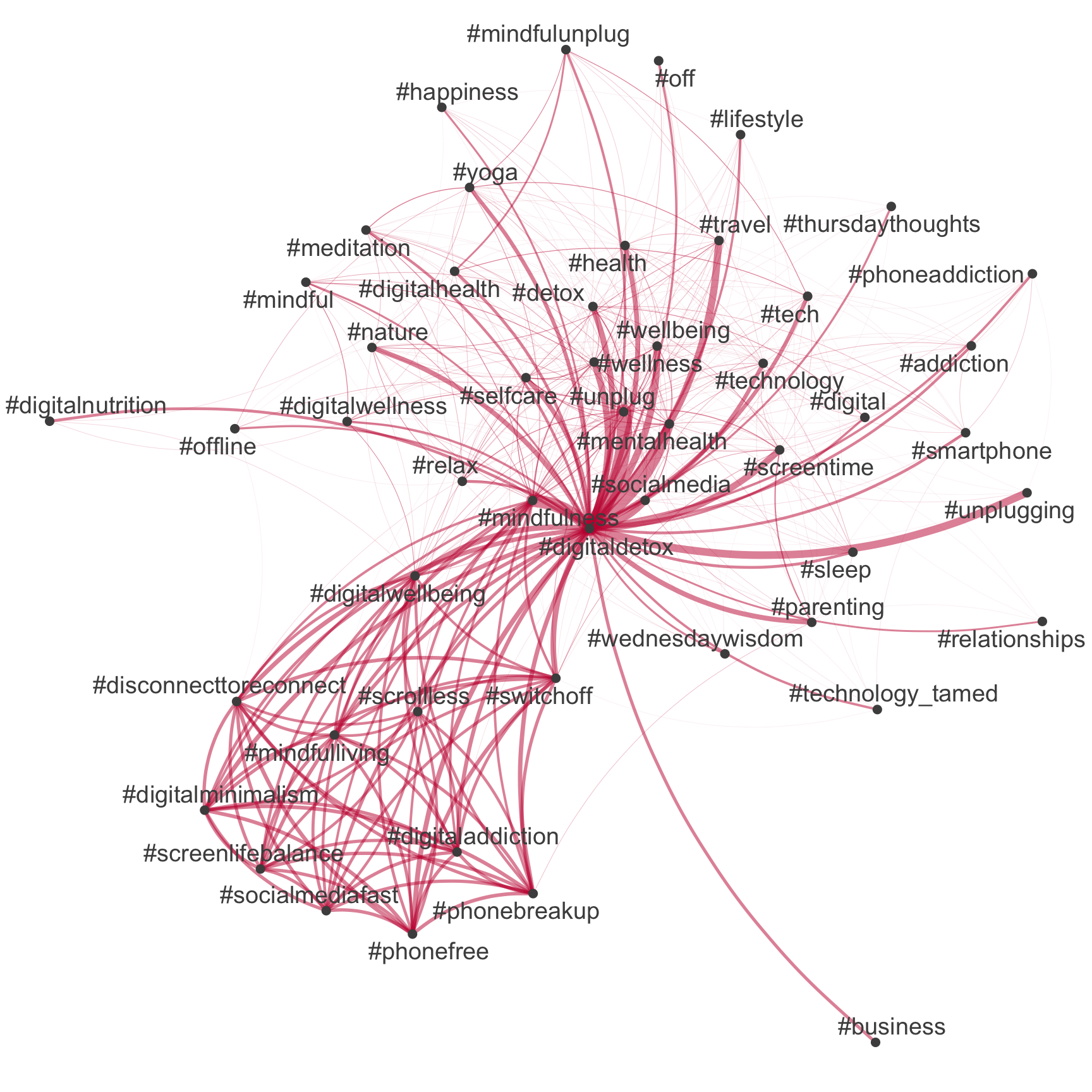
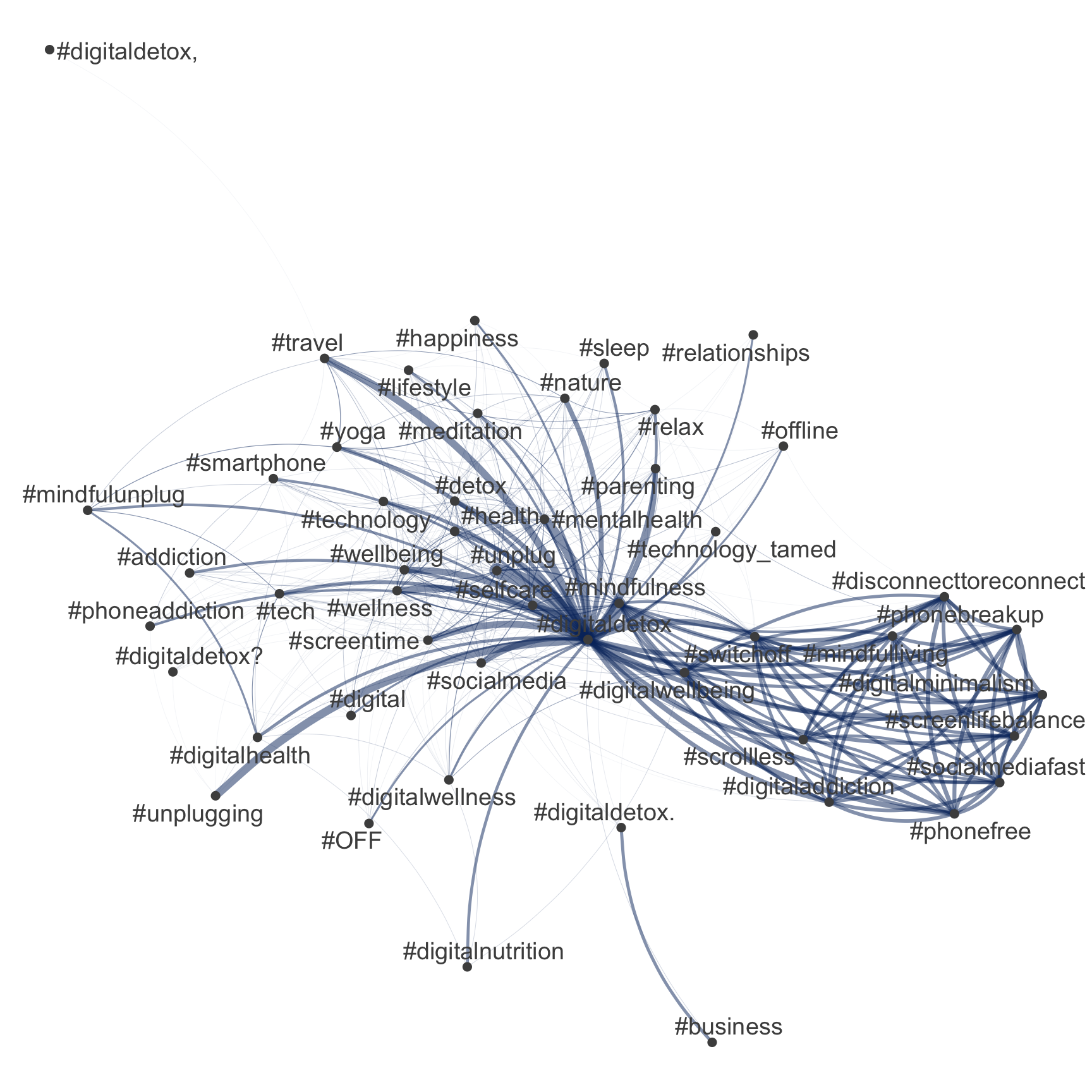
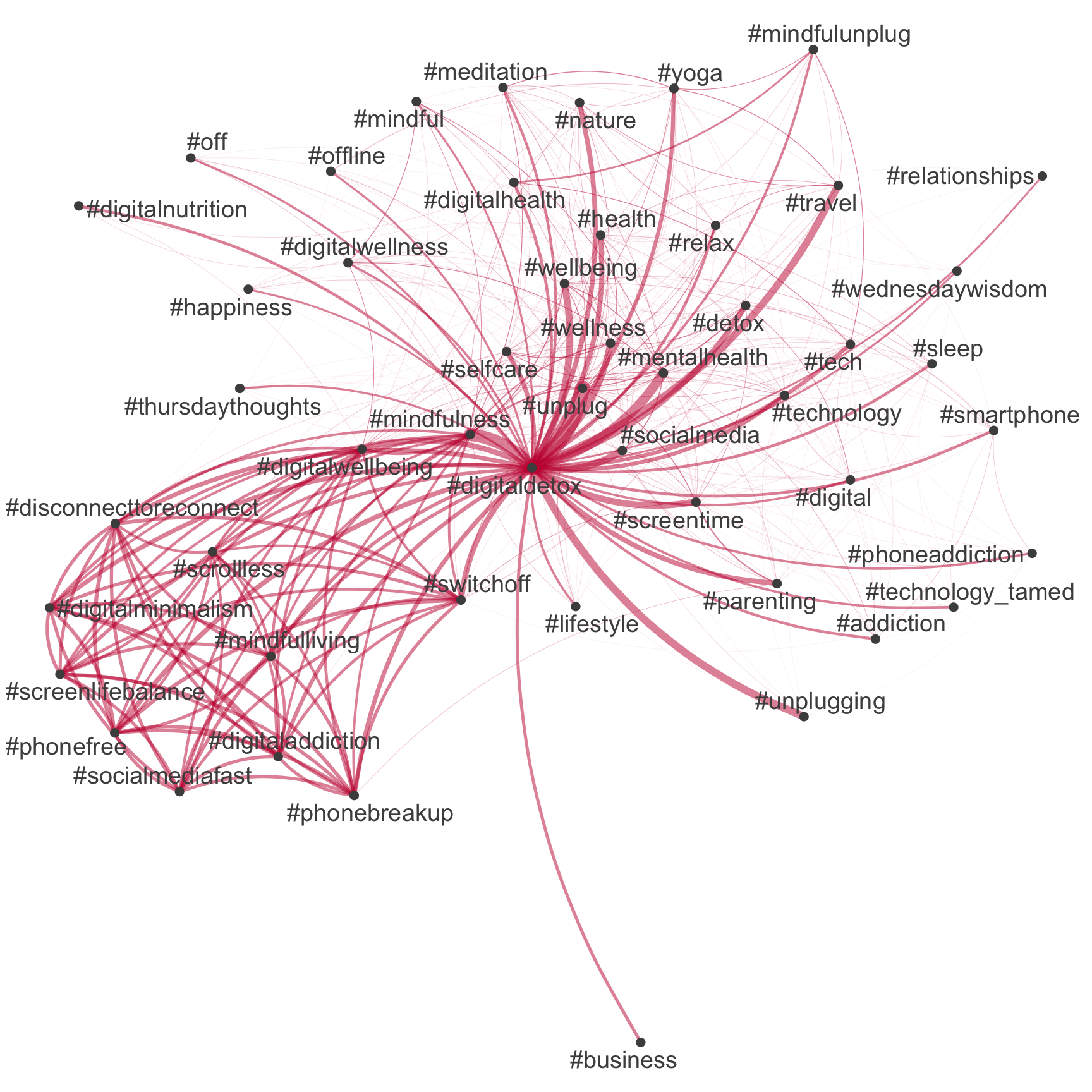
An example: Network of hashtags

Comparison between tidytext & quanteda

# Extract hashtags
tweets_hashtags <- tweets_detox %>% 
  mutate(hashtags = str_extract_all(
    text, "#\\S+")) %>%
  unnest(hashtags) 

# Extract most common hashtags
top50_hashtags_tidy <- tweets_hashtags %>% 
  count(hashtags, sort = TRUE) %>% 
  slice_head(n = 50) %>% 
  pull(hashtags)

# Visualize
tweets_hashtags %>% 
  count(tweet_id, hashtags, sort = TRUE) %>% 
  cast_dfm(tweet_id, hashtags, n) %>% 
  quanteda::fcm() %>% 
  quanteda::fcm_select(
    pattern = top50_hashtags_tidy,
    case_insensitive = FALSE
    ) %>% 
  quanteda.textplots::textplot_network(
    edge_color = "#04316A"
  )

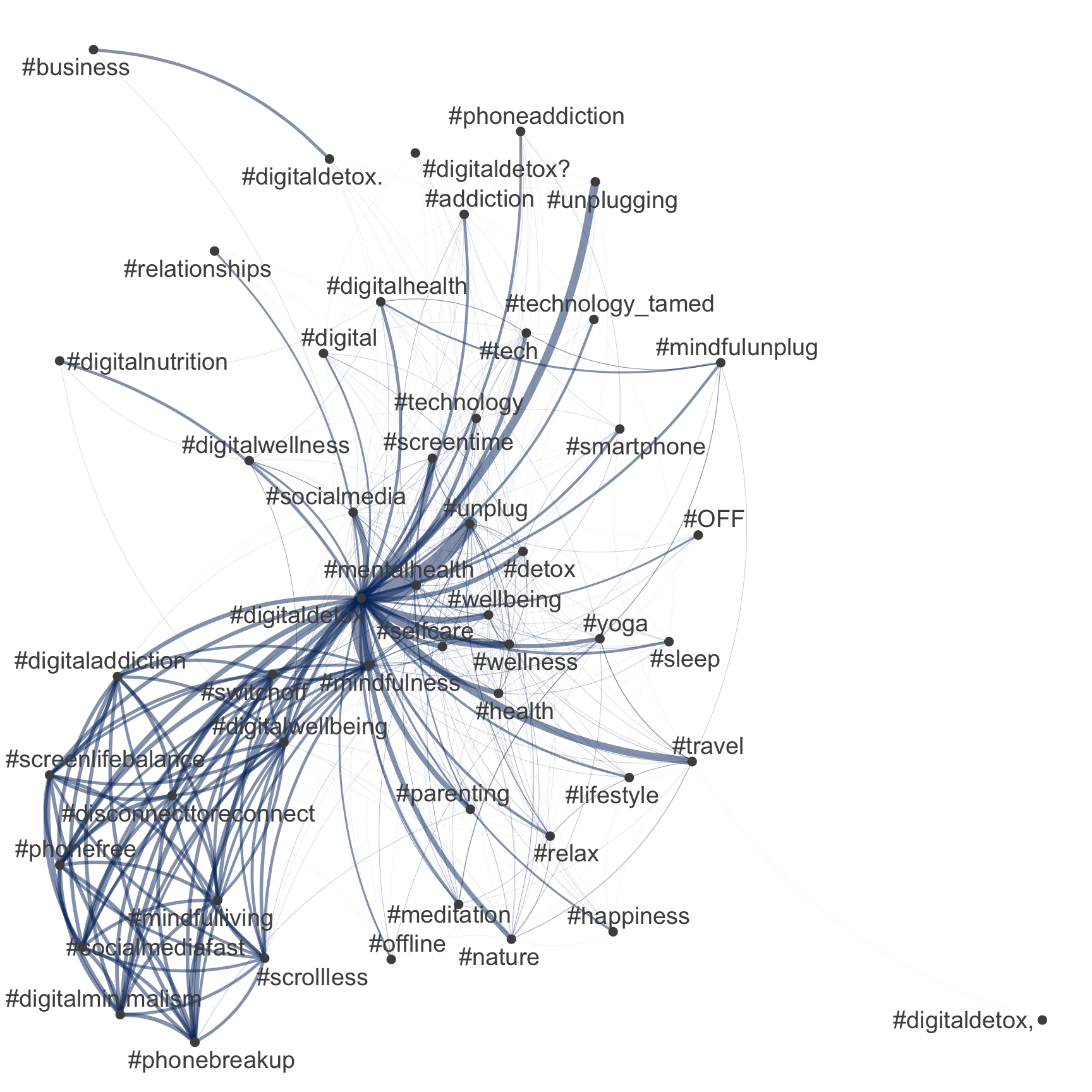
An example: Network of hashtags

Comparison between tidytext & quanteda

# Extract DFM with only hashtags
quanteda_dfm_hashtags <- quanteda_dfm %>% 
  quanteda::dfm_select(pattern = "#*") 

# Extract most common hashtags 
top50_hashtags_quanteda <- quanteda_dfm_hashtags %>% 
  topfeatures(50) %>% 
  names()

# Construct feature-occurrence matrix of hashtags
quanteda_dfm_hashtags %>% 
  fcm() %>% 
  fcm_select(pattern = top50_hashtags_quanteda) %>% 
  textplot_network(
    edge_color = "#C50F3C"
  )

An example: Network of hashtags

Comparison between tidytext & quanteda

Expand for full code

tweets_hashtags %>% 
  count(tweet_id, hashtags, sort = TRUE) %>% 
  cast_dfm(tweet_id, hashtags, n) %>% 
  quanteda::fcm() %>% 
  quanteda::fcm_select(
    pattern = top50_hashtags_tidy,
    case_insensitive = FALSE
    ) %>% 
  quanteda.textplots::textplot_network(
    edge_color = "#04316A"
  )

Expand for full code

quanteda_dfm_hashtags %>% 
  fcm() %>% 
  fcm_select(pattern = top50_hashtags_quanteda) %>% 
  textplot_network(
    edge_color = "#C50F3C"
  )

A new input in the pipeline

Unsupervised learning example: Topic modeling

Silge & Robinson (2017)

Building a shared vocabulary … again

Important terms and definitions

Topic Modeling: Form of unsupervised machine learning method used to exploratively identify topics in a corpus. Often, these are so-called mixed-membership models.
K: Number of topics to be calculated for a given a topic model.
Word-Topic-Matrix: Matrix describing the conditional probability (beta) with which a feature is prevalent in a given topic.
Document-Topic-Matrix: Matrix describing the conditional probability (gamma) with which a topic is prevalent in a given document.

Beyond LDA

Different topic modeling approaches

Latent Dirichlet Allocation [LDA] (Blei et al., 2003) is a probabilistic generative model that assumes each document in a corpus is a mix of topics and each word in the document is attributable to one of the document’s topics.
Structural Topic Modeling [STM] (Roberts et al., 2016; Roberts et al., 2019) extends LDA by incorporating document-level covariates, allowing for the modeling of how external factors influence topic prevalence.
Word embeddings (Word2Vec (Mikolov et al., 2013) , Glove (Pennington et al., 2014)) represent words as continuous vectors in a high-dimensional space, capturing semantic relationships between words based on their context in the data.
Topic Modeling with Neural Networks (BERTopic(Devlin et al., 2019), Doc2Vec(Le & Mikolov, 2014)) leverages deep learning architectures to automatically learn latent topics from textual data.

Preparation is everything

Suggested pre-processing steps (based on Maier et al. (2018))

⚠️ Deduplication;
✅ tokenization;
✅ transforming all characters to lowercase;
✅ removing punctuation and special characters;
✅ Removing stop-words;
⚠️ term unification (lemmatizing or stemming);
🏗️ relative pruning (attributed to Zipf’s law);

# Pruning
quanteda_dfm_trim <- quanteda_dfm %>% 
  dfm_trim( 
    min_docfreq = 10/nrow(tweets_detox),
    max_docfreq = 0.99, 
    docfreq_type = "prop")

# Convert for stm topic modeling
quanteda_stm <- quanteda_dfm_trim %>% 
   convert(to = "stm")

How to find K

The most important question of model selection

The choice of K (whether the model is instructed to identify 5, 15, or 100 topics), has a substantial impact on results:
- The smaller K, the more fine-grained and usually the more exclusive topics;
- the larger K, the more clearly topics identify individual events or issues.
The stm package (Roberts et al., 2019) has two build in solution to find the optimal K
- searchK() function
- setting K = 0 when estimating the model
Recommendation for stm: (Manual) training and evaluation!

Train and evaluate topic models

Better than `searchK()`: Manual exploration

# Set up parallel processing using furrr
future::plan(future::multisession()) 

# Estimate multiple models
stm_exploration <- tibble(
  k = seq(from = 5, to = 85, by = 5)
  ) %>%
  mutate(
    mdl = furrr::future_map(
      k, 
      ~stm::stm(
        documents = quanteda_stm$documents,
        vocab = quanteda_stm$vocab, 
        K = ., 
        seed = 42,
        max.em.its = 1000,
        init.type = "Spectral",
        verbose = FALSE),
    .options = furrr_options(seed = 42))
  )

stm_exploration$mdl

[[1]]
A topic model with 5 topics, 46574 documents and a 8268 word dictionary.

[[2]]
A topic model with 10 topics, 46574 documents and a 8268 word dictionary.

[[3]]
A topic model with 15 topics, 46574 documents and a 8268 word dictionary.

[[4]]
A topic model with 20 topics, 46574 documents and a 8268 word dictionary.

[[5]]
A topic model with 25 topics, 46574 documents and a 8268 word dictionary.

[[6]]
A topic model with 30 topics, 46574 documents and a 8268 word dictionary.

[[7]]
A topic model with 35 topics, 46574 documents and a 8268 word dictionary.

[[8]]
A topic model with 40 topics, 46574 documents and a 8268 word dictionary.

[[9]]
A topic model with 45 topics, 46574 documents and a 8268 word dictionary.

[[10]]
A topic model with 50 topics, 46574 documents and a 8268 word dictionary.

[[11]]
A topic model with 55 topics, 46574 documents and a 8268 word dictionary.

[[12]]
A topic model with 60 topics, 46574 documents and a 8268 word dictionary.

[[13]]
A topic model with 65 topics, 46574 documents and a 8268 word dictionary.

[[14]]
A topic model with 70 topics, 46574 documents and a 8268 word dictionary.

[[15]]
A topic model with 75 topics, 46574 documents and a 8268 word dictionary.

[[16]]
A topic model with 80 topics, 46574 documents and a 8268 word dictionary.

[[17]]
A topic model with 85 topics, 46574 documents and a 8268 word dictionary.

Semantic coherence as the key

Different model statistics for evaluation

Expand for full code

stm_results %>%
  transmute(
    k,
    `Lower bound` = lbound,
    Residuals = map_dbl(residual, "dispersion"),
    `Semantic coherence` = map_dbl(semantic_coherence, mean),
    `Held-out likelihood` = map_dbl(eval_heldout, "expected.heldout")) %>%
  gather(Metric, Value, -k) %>%
  ggplot(aes(k, Value, color = Metric)) +
    geom_line(size = 1.5, alpha = 0.7, show.legend = FALSE) +
    geom_point(size = 3) +
    scale_x_continuous(breaks = seq(from = 5, to = 85, by = 5)) +
    facet_wrap(~Metric, scales = "free_y") +
    labs(x = "K (number of topics)",
         y = NULL,
         title = "Model diagnostics by number of topics"
    ) +
    theme_pubr() +
    # add highlights 
    geom_vline(aes(xintercept =  5), color = "#00BFC4", alpha = .5) +
    geom_vline(aes(xintercept = 10), color = "#C77CFF", alpha = .5) +
    geom_vline(aes(xintercept = 40), color = "#C77CFF", alpha = .5)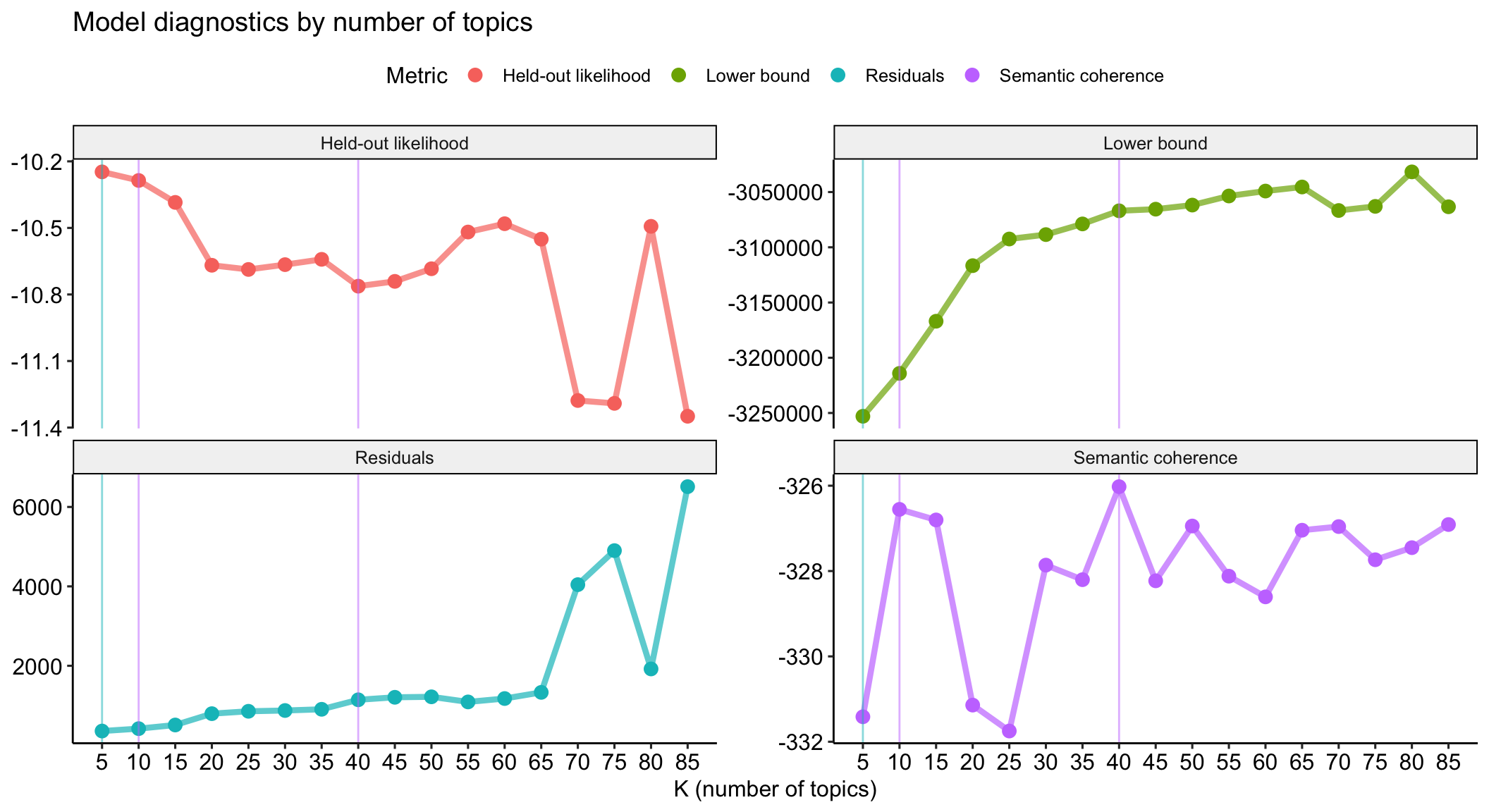

Finding the best trade-off

Comparison of selected models based on exclusivty and semantic coherence

Expand for full code

# Models for comparison
models_for_comparison = c(5, 10, 40)

# Create figures
stm_results %>% 
  # Edit data
  select(k, exclusivity, semantic_coherence) %>%
  filter(k %in% models_for_comparison) %>%
  unnest(cols = c(exclusivity, semantic_coherence))  %>%
  mutate(k = as.factor(k)) %>%
  # Build graph
  ggplot(aes(semantic_coherence, exclusivity, color = k)) +
    geom_point(size = 2, alpha = 0.7) +
    labs(
      x = "Semantic coherence",
      y = "Exclusivity"
      # title = "Comparing exclusivity and semantic coherence",
      # subtitle = "Models with fewer topics have higher semantic coherence for more topics, but lower exclusivity"
      ) +
    theme_pubr()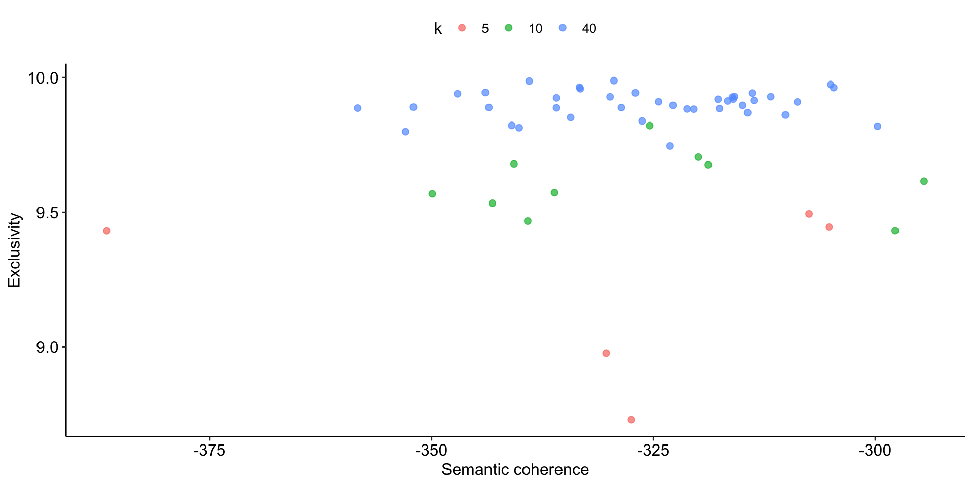

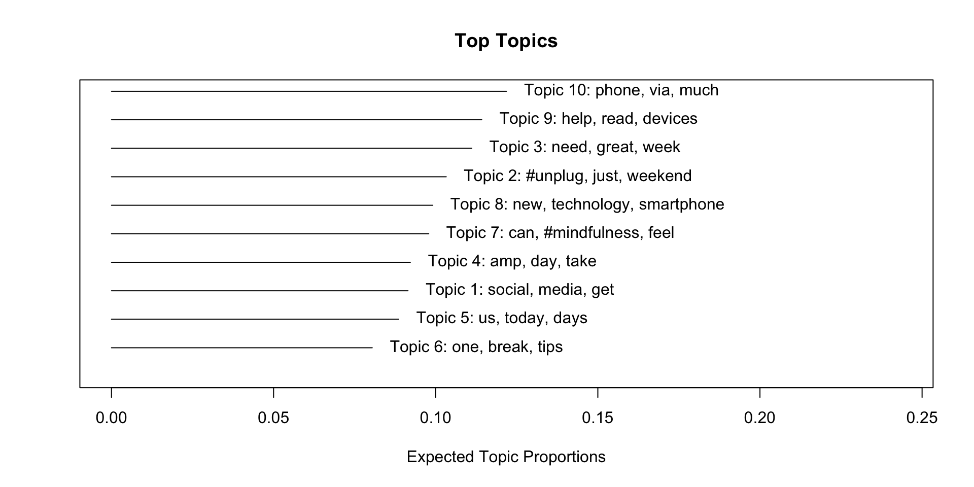
A first overview

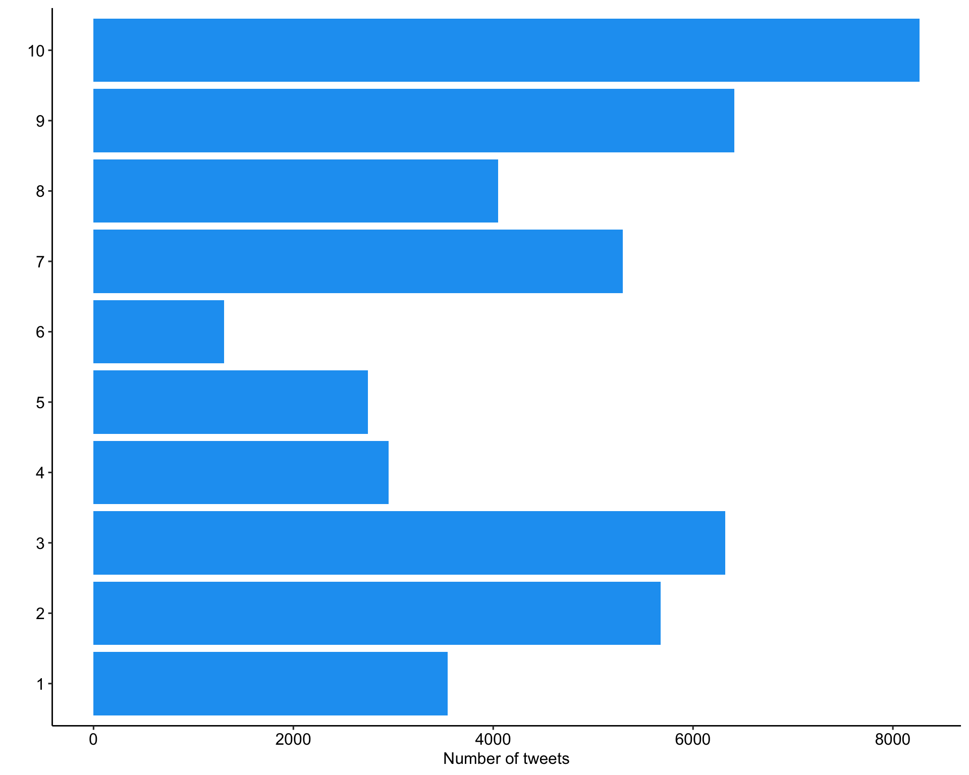
Understanding the ‘final’ model (k = 10)

tpm %>% plot(type = "summary")

A more detailed overview

Understanding the ‘final’ model (k = 10)

Expand for full code

# Create data
top_gamma <- tpm %>%
  tidy(matrix = "gamma") %>% 
  dplyr::group_by(topic) %>%
  dplyr::summarise(gamma = mean(gamma), .groups = "drop") %>%
  dplyr::arrange(desc(gamma))

top_beta <- tpm %>%
  tidytext::tidy(.) %>% 
  dplyr::group_by(topic) %>%
  dplyr::arrange(-beta) %>%
  dplyr::top_n(10, wt = beta) %>% 
  dplyr::select(topic, term) %>%
  dplyr::summarise(terms_beta = toString(term), .groups = "drop")

top_topics_terms <- top_beta %>% 
  dplyr::left_join(top_gamma, by = "topic") %>%
  dplyr::mutate(
          topic = reorder(topic, gamma)
      )

# Preview
top_topics_terms %>%
  mutate(across(gamma, ~round(.,3))) %>% 
  dplyr::arrange(-gamma) %>% 
  gt() %>% 
  cols_label(
    topic = "Topic", 
    terms_beta = "Top Terms (based on beta)",
    gamma = "Gamma"
  ) %>% 
  gtExtras::gt_theme_538()

Topic	Top Terms (based on beta)	Gamma
10	phone, via, much, #screentime, know, check, people, phones, #parenting, online	0.122
9	help, read, devices, use, world, tech, family, taking, kids, sleep	0.114
3	need, great, week, going, listen, #unplugging, discuss, @icphenomenallyu, away, well	0.111
2	#unplug, just, weekend, #travel, unplug, enjoy, #nature, really, join, nature	0.103
8	new, technology, smartphone, retreat, work, addiction, year, health, internet, without	0.099
7	can, #mindfulness, feel, #switchoff, #digitalwellbeing, #wellness, things, #phonefree, #disconnecttoreconnect, #digitalminimalism	0.098
4	amp, day, take, #mentalhealth, go, try, #wellbeing, now, give, every	0.092
1	social, media, get, life, back, like, good, #socialmedia, find, see	0.091
5	us, today, days, next, put, happy, may, facebook, share, hour	0.089
6	one, break, tips, make, screen, love, #technology, free, looking, getting	0.080

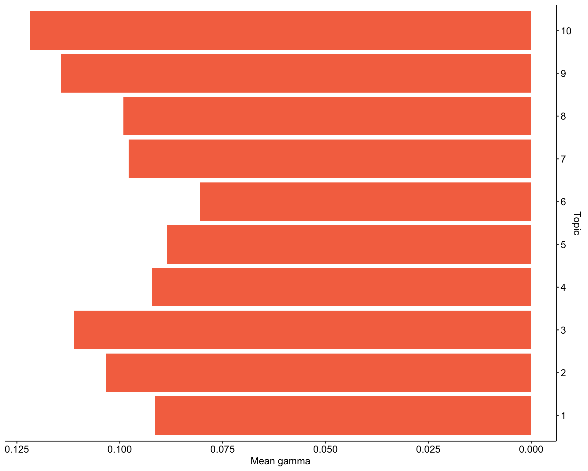
Results in a different context

Merge back with original data for further analysis and comparison

top_gamma %>% 
  ggplot(aes(as.factor(topic), gamma)) +
  geom_col(fill = "#F57350") +
  labs(
    x = "Topic",
    y = "Mean gamma"
  ) +
  coord_flip() +
  scale_y_reverse() +
  scale_x_discrete(position = "top") +
  theme_pubr()
tweets_detox_topics %>% 
  mutate(across(top_topic, as.factor)) %>% 
  ggplot(aes(top_topic)) +
  geom_bar(fill = "#1DA1F2") +
  labs(
    x = "", 
    y = "Number of tweets"
  ) +
  coord_flip() +
  theme_pubr()

Expand for full code

Most representative tweets for Topic 10

Check interpretability and relevance of topics

Expand for full code

tweets_detox_topics %>% 
  filter(top_topic == 10) %>% 
  arrange(-top_gamma) %>% 
  slice_head(n = 10) %>% 
  select(tweet_id, user_username, created_at, text, top_gamma) %>% 
  gt() %>% 
  gtExtras::gt_theme_538() %>% 
  gt::tab_options(table.font.size = "10px")

tweet_id	user_username	created_at	text	top_gamma
1496707135794827266	beckygrantstr	2022-02-24 04:42:43	Do you have a blind spot when it comes to what your kids are doing online? #screentime #parenting #digitaldetox Parents Have a Blind Spot When it Comes to Kids and Screens \| by Becky Grant \| A Parent Is Born \| Feb, 2022 \| Medium - via @pensignal https://t.co/EcV7yKn4WX	0.8192142
1496343978672898048	beckygrantstr	2022-02-23 04:39:39	Do you have a blind spot when it comes to what your kids are doing online? #screentime #parenting #digitaldetox Parents Have a Blind Spot When it Comes to Kids and Screens \| by Becky Grant \| A Parent Is Born \| Feb, 2022 \| Medium - via @pensignal https://t.co/o9e6WQIpm5	0.8192142
1495981434665947137	beckygrantstr	2022-02-22 04:39:02	Do you have a blind spot when it comes to what your kids are doing online? #screentime #parenting #digitaldetox Parents Have a Blind Spot When it Comes to Kids and Screens \| by Becky Grant \| A Parent Is Born \| Feb, 2022 \| Medium - via @pensignal https://t.co/rQgcPltrMt	0.8192142
1499612427503247360	beckygrantstr	2022-03-04 05:07:18	Do you have a blind spot when it comes to what your kids are doing online? #screentime #parenting #digitaldetox Parents Have a Blind Spot When it Comes to Kids and Screens \| by Becky Grant \| A Parent Is Born \| Feb, 2022 \| Medium - via @pensignal https://t.co/DQRQlN1iyq	0.8192142
1499249315381977089	beckygrantstr	2022-03-03 05:04:26	Do you have a blind spot when it comes to what your kids are doing online? #screentime #parenting #digitaldetox Parents Have a Blind Spot When it Comes to Kids and Screens \| by Becky Grant \| A Parent Is Born \| Feb, 2022 \| Medium - via @pensignal https://t.co/L7ly66J2fq	0.8192142
1498886117394980865	beckygrantstr	2022-03-02 05:01:13	Do you have a blind spot when it comes to what your kids are doing online? #screentime #parenting #digitaldetox Parents Have a Blind Spot When it Comes to Kids and Screens \| by Becky Grant \| A Parent Is Born \| Feb, 2022 \| Medium - via @pensignal https://t.co/uJPIMYY1Id	0.8192142
1498522796611321864	beckygrantstr	2022-03-01 04:57:30	Do you have a blind spot when it comes to what your kids are doing online? #screentime #parenting #digitaldetox Parents Have a Blind Spot When it Comes to Kids and Screens \| by Becky Grant \| A Parent Is Born \| Feb, 2022 \| Medium - via @pensignal https://t.co/z4Fv2bmeag	0.8192142
1498159674008510465	beckygrantstr	2022-02-28 04:54:35	Do you have a blind spot when it comes to what your kids are doing online? #screentime #parenting #digitaldetox Parents Have a Blind Spot When it Comes to Kids and Screens \| by Becky Grant \| A Parent Is Born \| Feb, 2022 \| Medium - via @pensignal https://t.co/SdZFAJy6kZ	0.8192142
1497796525929472003	beckygrantstr	2022-02-27 04:51:34	Do you have a blind spot when it comes to what your kids are doing online? #screentime #parenting #digitaldetox Parents Have a Blind Spot When it Comes to Kids and Screens \| by Becky Grant \| A Parent Is Born \| Feb, 2022 \| Medium - via @pensignal https://t.co/OKLMzwfQUA	0.8192142
1497433419512524802	beckygrantstr	2022-02-26 04:48:42	Do you have a blind spot when it comes to what your kids are doing online? #screentime #parenting #digitaldetox Parents Have a Blind Spot When it Comes to Kids and Screens \| by Becky Grant \| A Parent Is Born \| Feb, 2022 \| Medium - via @pensignal https://t.co/yTnqhTPV8h	0.8192142

Users with most tweets about Topic 10

Check interpretability and relevance of topics

tweets_detox_topics %>% 
  filter(top_topic == 10) %>% 
  count(user_username, sort = TRUE) %>% 
  mutate(
    prop = round(n/sum(n)*100, 2)) %>% 
  slice_head(n = 10) %>% 
  gt() %>% 
  gtExtras::gt_theme_538()

user_username	n	prop
TimeToLogOff	2384	28.83
punkt	390	4.72
petitstvincent	175	2.12
tanyagoodin	135	1.63
ditox_unplug	111	1.34
OurHourOff	99	1.20
beckygrantstr	63	0.76
CreeEscape	56	0.68
ConsciDigital	51	0.62
phubboo	50	0.60

Validate, validate, validate!

Things to remember about topic models

topic models are a useful tool for automated content analysis, both when exploring a large amount of data and when it comes to systematically identifying relationships between topics and other variables
certain prerequisites such as minimum size and variety of the corpus (namely on the level of words and documents and their relation to each other) need to be met for a conclusive model
everything above a certain degree of word frequencies is considered a “topic,” even if it is not a topic in human interpretation
Reading the tea leaves (Chang et al., 2009) or (again): validate, validate, validate (e.g. with oolong package (Chan & Sältzer, 2020))

📋 Hands on working with R

Various exercises on the content of today’s session

🧪 And now … you: Model away!

Objective of this exercise

Brief review of the contents of the last session
Teaching the basic steps for creating and analyzing document feature matrices and stm topic models

Next steps

Download files provided on StudOn or shared drives for the sessions
Unzip the archive at a destination of your choice.
Double click on the Exercise-Automatic_text_analysis.Rproj to open the RStudio project. This ensures that all dependencies are working correctly.
Open the exercise.qmd file and follow the instructions.
Tip: You can find all code chunks used in the slides in the showcase.qmd (for the raw code) or showcase.html (with rendered outputs).

Time for questions

Thank you!

References

Barrie, C., & Ho, J. (2021). academictwitteR: An r package to access the twitter academic research product track v2 API endpoint. Journal of Open Source Software, 6(62), 3272. https://doi.org/10.21105/joss.03272

Blei, D. M., Ng, A. Y., & Jordan, M. I. (2003). Latent dirichlet allocation. The Journal of Machine Learning Research, 3, 9931022.

Chan, C., & Sältzer, M. (2020). Oolong: An r package for validating automated content analysis tools. Journal of Open Source Software, 5(55), 2461. https://doi.org/10.21105/joss.02461

Chang, J., Boyd-Graber, J., Gerrish, S., Wang, C., & Blei, D. (2009). Reading tea leaves: How humans interpret topic models. 32, 288–296.

Devlin, J., Chang, M.-W., Lee, K., & Toutanova, K. (2019). BERT: Pre-training of deep bidirectional transformers for language understanding (J. Burstein, C. Doran, & T. Solorio, Eds.; p. 41714186). Association for Computational Linguistics. https://doi.org/10.18653/v1/N19-1423

Le, Q., & Mikolov, T. (2014). Distributed representations of sentences and documents (E. P. Xing & T. Jebara, Eds.; Vol. 32, p. 11881196). PMLR. https://proceedings.mlr.press/v32/le14.html

Maier, D., Waldherr, A., Miltner, P., Wiedemann, G., Niekler, A., Keinert, A., Pfetsch, B., Heyer, G., Reber, U., Häussler, T., Schmid-Petri, H., & Adam, S. (2018). Applying LDA Topic Modeling in Communication Research: Toward a Valid and Reliable Methodology. Communication Methods and Measures, 12(2-3), 93–118. https://doi.org/10.1080/19312458.2018.1430754

Mikolov, T., Sutskever, I., Chen, K., Corrado, G. S., & Dean, J. (2013). Distributed representations of words and phrases and their compositionality (C. J. Burges, L. Bottou, M. Welling, Z. Ghahramani, & K. Q. Weinberger, Eds.; Vol. 26). Curran Associates, Inc. https://proceedings.neurips.cc/paper_files/paper/2013/file/9aa42b31882ec039965f3c4923ce901b-Paper.pdf

Pennington, J., Socher, R., & Manning, C. D. (2014). Glove: Global vectors for word representation. 15321543. https://doi.org/10.3115/v1/D14-1162

Roberts, M. E., Stewart, B. M., & Airoldi, E. M. (2016). A model of text for experimentation in the social sciences. Journal of the American Statistical Association, 111(515), 988–1003. https://doi.org/f88tzh

Roberts, M. E., Stewart, B. M., & Tingley, D. (2019). stm: An R Package for Structural Topic Models. Journal of Statistical Software, 91(1), 1–40. https://doi.org/10.18637/jss.v091.i02

Silge, J., & Robinson, D. (2017). Text mining with r: A tidy approach (First edition). O’Reilly.

Zheng, A., & Casari, A. (2018). Feature engineering for machine learning: Principles and techniques for data scientists (First edition). O’Reilly.

🔨 Automatic text analysis in R

print("Hello (again)!")

Schedule

Agenda

What we did so far

Social Media as 💊, 👹 or 🍩 ?

Discussion about digital disconnection on twitter

The tidy text format pipeline basics

Focus on single words and their relationship documents & sentiments

Text as data in R

Expansion of the pipeline

Focus on modeling the realtionships between words & documents

Quick recap on Document-Term Matrix [DTM]

Most common structure for (classic) text mining

Step-by-step DTM creation

Along the tidy text pipeline: Tokenize

Step-by-step DTM creation

Along the tidy text pipeline: Tokenize ▶️ Summarize

Step-by-step DTM creation

Along the tidy text pipeline: Tokenize ▶️ Summarize ▶️ DTM

Choose or combine styles

Simple with tidytext, precise with quanteda

An example: Network of hashtags

Comparison between tidytext & quanteda

An example: Network of hashtags

Comparison between tidytext & quanteda

An example: Network of hashtags

Comparison between tidytext & quanteda

A new input in the pipeline

Unsupervised learning example: Topic modeling

Building a shared vocabulary … again

Important terms and definitions

Beyond LDA

Different topic modeling approaches

Preparation is everything

Suggested pre-processing steps (based on Maier et al. (2018))

How to find K

The most important question of model selection

Train and evaluate topic models

Better than searchK(): Manual exploration

Semantic coherence as the key

Different model statistics for evaluation

Finding the best trade-off

Comparison of selected models based on exclusivty and semantic coherence

A first overview

Understanding the ‘final’ model (k = 10)

A more detailed overview

Understanding the ‘final’ model (k = 10)

Results in a different context

Merge back with original data for further analysis and comparison

Most representative tweets for Topic 10

Check interpretability and relevance of topics

Users with most tweets about Topic 10

Check interpretability and relevance of topics

Validate, validate, validate!

Things to remember about topic models

📋 Hands on working with R

🧪 And now … you: Model away!

Next steps

Time for questions

Thank you!

References

`print("Hello (again)!")`

Better than `searchK()`: Manual exploration