Unsupervised Machine Learning II

Session 10 - Showcase

Published

13.01.2025

Link to slides

Preparation

if (!require("pacman")) install.packages("pacman")
pacman::p_load(
    here, qs, # file management
    magrittr, janitor, # data wrangling
    easystats, sjmisc, # data analysis
    gt, gtExtras, # table visualization
    ggpubr, ggwordcloud, # visualization
    # text analysis    
    tidytext, widyr, # based on tidytext
    quanteda, # based on quanteda
    quanteda.textmodels, quanteda.textplots, quanteda.textstats, 
    stm, # structural topic modeling
    openalexR, pushoverr, tictoc, 
    tidyverse # load last to avoid masking issues
  )

review_works <- qs::qread(here("data/session-07/openalex-review_works-2013_2023.qs"))

# Create correct data
review_subsample <- review_works %>% 
    # Create additional factor variables
    mutate(
        publication_year_fct = as.factor(publication_year), 
        type_fct = as.factor(type)
        ) %>%
    # Eingrenzung: Sprache und Typ
    filter(language == "en") %>% 
    filter(type == "article") %>%
    # Datentranformation
    unnest(topics, names_sep = "_") %>%
    filter(topics_name == "field") %>% 
    filter(topics_i == "1") %>% 
    # Eingrenzung: Forschungsfeldes
    filter(
    topics_display_name == "Social Sciences"|
    topics_display_name == "Psychology"
    ) %>% 
    mutate(
        field = as.factor(topics_display_name)
    ) %>% 
    # Eingrenzung: Keine Einträge ohne Abstract
    filter(!is.na(ab))

# Create corpus
quanteda_corpus <- review_subsample %>% 
  quanteda::corpus(
    docid_field = "id", 
    text_field = "ab"
  )

# Tokenize
quanteda_token <- quanteda_corpus %>% 
  quanteda::tokens(
    remove_punct = TRUE,
    remove_symbols = TRUE, 
    remove_numbers = TRUE, 
    remove_url = TRUE, 
    split_tags = FALSE # keep hashtags and mentions
  ) %>% 
  quanteda::tokens_tolower() %>% 
  quanteda::tokens_remove(
    pattern = stopwords("en")
    )

# Convert to Document-Feature-Matrix (DFM)
quanteda_dfm <- quanteda_token %>% 
  quanteda::dfm()

# Pruning
quanteda_dfm_trim <- quanteda_dfm %>% 
  dfm_trim( 
    min_docfreq = 10/nrow(review_subsample),
    max_docfreq = 0.99, 
    docfreq_type = "prop")

# Convert for stm topic modeling
quanteda_stm <- quanteda_dfm_trim %>% 
   convert(to = "stm")

Codechunks aus der Sitzung

(Re-)Estimation of k = 20 with metadata

# Estimate model
stm_mdl_k20 <- stm::stm(
    documents = quanteda_stm$documents,
    vocab = quanteda_stm$vocab, 
    prevalence =~ publication_year_fct + field, 
    K = 20, 
    seed = 42,
    max.em.its = 1000,
    data = quanteda_stm$meta,
    init.type = "Spectral",
    verbose = TRUE)

# Overview
stm_mdl_k20

A topic model with 20 topics, 36650 documents and a 14322 word dictionary.

Erweiterte Auswertungen

Beta-Matrix

# Create tidy beta matrix
td_beta <- tidy(stm_mdl_k20)

# Output 
td_beta

# A tibble: 286,440 × 3
   topic term      beta
   <int> <chr>    <dbl>
 1     1 #x0d  6.83e-44
 2     2 #x0d  2.37e-30
 3     3 #x0d  3.35e-45
 4     4 #x0d  7.24e- 3
 5     5 #x0d  1.45e-23
 6     6 #x0d  5.23e-20
 7     7 #x0d  2.70e-12
 8     8 #x0d  3.32e-39
 9     9 #x0d  8.78e- 4
10    10 #x0d  2.58e-12
# ℹ 286,430 more rows

# Create top terms
top_terms <- td_beta %>%
  arrange(beta) %>%
  group_by(topic) %>%
  top_n(7, beta) %>%
  arrange(-beta) %>%
  select(topic, term) %>%
  summarise(terms = list(term)) %>%
  mutate(terms = map(terms, paste, collapse = ", ")) %>% 
  unnest(cols = c(terms))

# Output
top_terms

# A tibble: 20 × 2
   topic terms                                                                  
   <int> <chr>                                                                  
 1     1 sleep, studies, eating, cognitive, weight, associated, duration        
 2     2 health, women, gender, cultural, barriers, men, countries              
 3     3 treatment, disorders, symptoms, disorder, depression, anxiety, therapy 
 4     4 patients, cancer, nurses, patient, music, nursing, pain                
 5     5 literature, university, author, gt, lt, et, al                         
 6     6 prevalence, covid-19, suicide, pandemic, studies, among, risk          
 7     7 articles, review, study, systematic, results, search, science          
 8     8 physical, activity, disabilities, exercise, cognitive, adults, body    
 9     9 learning, education, students, educational, skills, teachers, teaching 
10    10 de, la, y, en, los, 的, el                                             
11    11 work, study, development, can, public, management, factors             
12    12 violence, sexual, use, abuse, risk, youth, h3                          
13    13 health, mental, care, support, people, social, family                  
14    14 social, use, media, digital, information, technology, communication    
15    15 ci, effect, meta-analysis, p, studies, effects, trials                 
16    16 research, literature, review, future, findings, systematic, paper      
17    17 children, studies, factors, relationship, adolescents, review, associa…
18    18 measures, assessment, used, studies, tools, measurement, quality       
19    19 studies, interventions, included, evidence, review, systematic, outcom…
20    20 programs, school, training, interventions, outcomes, review, intervent…

td_beta %>%
    group_by(topic) %>%
    slice_max(beta, n = 10) %>%
    ungroup() %>%
    ggplot(aes(beta, term)) +
    geom_col() +
    facet_wrap(~ topic, scales = "free")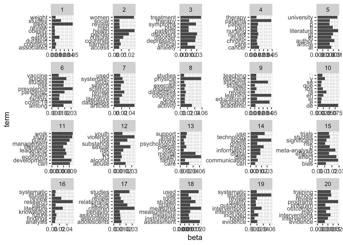

Gamma-Matrix

# Create tidy gamma matrix
td_gamma <- tidy(
  stm_mdl_k20, 
  matrix = "gamma", 
  document_names = names(quanteda_stm$documents)
  )

# Output 
td_gamma

# A tibble: 733,000 × 3
   document                         topic    gamma
   <chr>                            <int>    <dbl>
 1 https://openalex.org/W4293003987     1 0.00473 
 2 https://openalex.org/W2750168540     1 0.000270
 3 https://openalex.org/W1998933811     1 0.00368 
 4 https://openalex.org/W2547134104     1 0.00340 
 5 https://openalex.org/W3047898105     1 0.00263 
 6 https://openalex.org/W2149640470     1 0.00230 
 7 https://openalex.org/W2740726397     1 0.0374  
 8 https://openalex.org/W2974087526     1 0.00339 
 9 https://openalex.org/W2195703978     1 0.00287 
10 https://openalex.org/W2093916237     1 0.170   
# ℹ 732,990 more rows

Häufigkeit und Top Begriffe der Themen

prevalence <- td_gamma %>%
  group_by(topic) %>%
  summarise(gamma = mean(gamma)) %>%
  arrange(desc(gamma)) %>%
  left_join(top_terms, by = "topic") %>%
  mutate(topic = paste0("Topic ",sprintf("%02d", topic)),
         topic = reorder(topic, gamma))

Table

prevalence %>% 
  gt() %>% 
  fmt_number(
    columns = c(gamma), 
    decimals = 2) %>% 
  gtExtras::gt_theme_538()

topic	gamma	terms
Topic 16	0.12	research, literature, review, future, findings, systematic, paper
Topic 19	0.09	studies, interventions, included, evidence, review, systematic, outcomes
Topic 07	0.08	articles, review, study, systematic, results, search, science
Topic 11	0.07	work, study, development, can, public, management, factors
Topic 09	0.06	learning, education, students, educational, skills, teachers, teaching
Topic 17	0.06	children, studies, factors, relationship, adolescents, review, associated
Topic 13	0.06	health, mental, care, support, people, social, family
Topic 14	0.05	social, use, media, digital, information, technology, communication
Topic 15	0.05	ci, effect, meta-analysis, p, studies, effects, trials
Topic 03	0.04	treatment, disorders, symptoms, disorder, depression, anxiety, therapy
Topic 06	0.04	prevalence, covid-19, suicide, pandemic, studies, among, risk
Topic 18	0.04	measures, assessment, used, studies, tools, measurement, quality
Topic 20	0.04	programs, school, training, interventions, outcomes, review, intervention
Topic 02	0.04	health, women, gender, cultural, barriers, men, countries
Topic 01	0.03	sleep, studies, eating, cognitive, weight, associated, duration
Topic 05	0.03	literature, university, author, gt, lt, et, al
Topic 12	0.03	violence, sexual, use, abuse, risk, youth, h3
Topic 04	0.03	patients, cancer, nurses, patient, music, nursing, pain
Topic 08	0.03	physical, activity, disabilities, exercise, cognitive, adults, body
Topic 10	0.00	de, la, y, en, los, 的, el

Visualization

prevalence %>%
  ggplot(aes(topic, gamma, label = terms, fill = topic)) +
  geom_col(show.legend = FALSE) +
  geom_text(hjust = 0, nudge_y = 0.0005, size = 3) +
  coord_flip() +
  scale_y_continuous(
    expand = c(0,0),
    limits = c(0, 0.18)) +
  theme_pubr() +
  theme(
    plot.title = element_text(size = 16),
    plot.subtitle = element_text(size = 13)) +
  labs(
    x = NULL, y = expression(gamma),
    title = "Topic Prevalence in the OpenAlex Corpus",
    subtitle = "With the top seven words that contribute to each topic")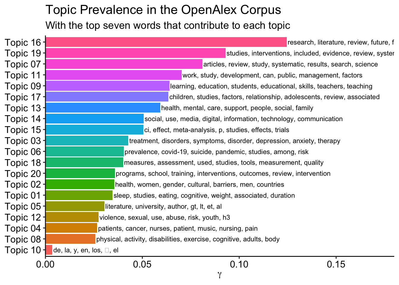

Effect metadata

effects <- estimateEffect(
  1:20 ~ publication_year_fct + field, 
  stm_mdl_k20, 
  meta = quanteda_stm$meta)

# Comparison
# Effects of covariates on Topic 6
effects %>% summary(topics = 6)


Call:
estimateEffect(formula = 1:20 ~ publication_year_fct + field, 
    stmobj = stm_mdl_k20, metadata = quanteda_stm$meta)


Topic 6:

Coefficients:
                          Estimate Std. Error t value Pr(>|t|)    
(Intercept)               0.039537   0.004317   9.158  < 2e-16 ***
publication_year_fct2014 -0.001672   0.005739  -0.291  0.77077    
publication_year_fct2015 -0.002156   0.005404  -0.399  0.68984    
publication_year_fct2016 -0.003294   0.005365  -0.614  0.53916    
publication_year_fct2017 -0.002819   0.005349  -0.527  0.59818    
publication_year_fct2018 -0.004524   0.004996  -0.905  0.36522    
publication_year_fct2019 -0.001295   0.004712  -0.275  0.78339    
publication_year_fct2020  0.006487   0.004891   1.326  0.18481    
publication_year_fct2021  0.023181   0.004826   4.803 1.57e-06 ***
publication_year_fct2022  0.025637   0.004629   5.538 3.07e-08 ***
publication_year_fct2023  0.013614   0.004450   3.059  0.00222 ** 
fieldSocial Sciences     -0.010482   0.001634  -6.416 1.42e-10 ***
---
Signif. codes:  0 '***' 0.001 '**' 0.01 '*' 0.05 '.' 0.1 ' ' 1

# Effects of covariates on Topic 16
effects %>% summary(topics = 16)


Call:
estimateEffect(formula = 1:20 ~ publication_year_fct + field, 
    stmobj = stm_mdl_k20, metadata = quanteda_stm$meta)


Topic 16:

Coefficients:
                          Estimate Std. Error t value Pr(>|t|)    
(Intercept)               0.063763   0.004937  12.917   <2e-16 ***
publication_year_fct2014  0.007002   0.006553   1.068   0.2853    
publication_year_fct2015  0.012720   0.006291   2.022   0.0432 *  
publication_year_fct2016  0.004582   0.006161   0.744   0.4571    
publication_year_fct2017  0.006917   0.006132   1.128   0.2593    
publication_year_fct2018  0.002035   0.006282   0.324   0.7460    
publication_year_fct2019 -0.001197   0.005717  -0.209   0.8342    
publication_year_fct2020  0.002731   0.005628   0.485   0.6275    
publication_year_fct2021  0.002666   0.005397   0.494   0.6214    
publication_year_fct2022 -0.001183   0.005321  -0.222   0.8241    
publication_year_fct2023  0.008051   0.005285   1.524   0.1276    
fieldSocial Sciences      0.086250   0.001807  47.743   <2e-16 ***
---
Signif. codes:  0 '***' 0.001 '**' 0.01 '*' 0.05 '.' 0.1 ' ' 1

effects %>%
  tidy() %>% 
  filter(
    term != "(Intercept)",
    term == "fieldSocial Sciences") %>% 
    select(-term) %>% 
  gt() %>% 
    fmt_number(
      columns = -c(topic),
      decimals = 3
    ) %>% 
  # Color social science topics "blue"
  data_color(
    columns = topic,
    rows = estimate > 0,
    method = "numeric",
    palette = c("#04316A"),
    alpha = 0.4
  ) %>% 
  # Color psychology topics "yellow"
  data_color(
    columns = topic,
    rows = estimate < 0,
    method = "numeric",
    palette = c("#D3A518"),
    alpha = 0.4
  ) %>% 
  # # Color effect size for estimation
  # data_color(
  #   columns = estimate,
  #   method = "numeric",
  #   palette = "viridis"
  # ) %>% 
  # # Color insignificant p-values
  # data_color(
  #   columns = p.value,
  #   rows = p.value > 0.05,
  #   method = "numeric",
  #   palette = c("#C50F3C", "#C50F3C")
  # ) %>% 
  gtExtras::gt_theme_538()

topic	estimate	std.error	statistic	p.value
1	−0.056	0.001	−38.174	0.000
2	0.014	0.001	10.475	0.000
3	−0.069	0.001	−52.240	0.000
4	−0.014	0.001	−11.334	0.000
5	0.027	0.001	19.297	0.000
6	−0.010	0.002	−6.504	0.000
7	0.014	0.001	11.993	0.000
8	−0.015	0.001	−13.266	0.000
9	0.053	0.002	28.392	0.000
10	−0.002	0.001	−2.695	0.007
11	0.091	0.002	56.520	0.000
12	0.003	0.001	2.282	0.022
13	−0.025	0.001	−17.476	0.000
14	0.044	0.002	29.100	0.000
15	−0.059	0.001	−39.576	0.000
16	0.086	0.002	47.525	0.000
17	−0.033	0.001	−23.901	0.000
18	−0.012	0.001	−11.532	0.000
19	−0.044	0.001	−33.348	0.000
20	0.008	0.001	7.621	0.000

Zusammenführung der Daten

Merge mit Stammdaten

gamma_export <- stm_mdl_k20 %>% 
  tidytext::tidy(
    matrix = "gamma", 
    document_names = names(quanteda_stm$documents)) %>%
  dplyr::group_by(document) %>% 
  dplyr::slice_max(gamma) %>% 
  dplyr::mutate(main_topic = ifelse(gamma > 0.5, topic, NA)) %>% 
      rename(
        top_topic = topic,
        top_gamma = gamma) %>% 
  dplyr::ungroup() %>% 
  dplyr::left_join(review_subsample, by = c("document" = "id")) %>% 
  dplyr::rename(id = document) %>% 
  dplyr::mutate(
    stm_topic = as.factor(paste("Topic", sprintf("%02d", top_topic)))
  )

Anzahl der Abstracts nach Thema

gamma_export %>% 
  ggplot(aes(x = fct_rev(fct_infreq(stm_topic)))) +
  geom_bar() +
  coord_flip() +
  theme_pubr()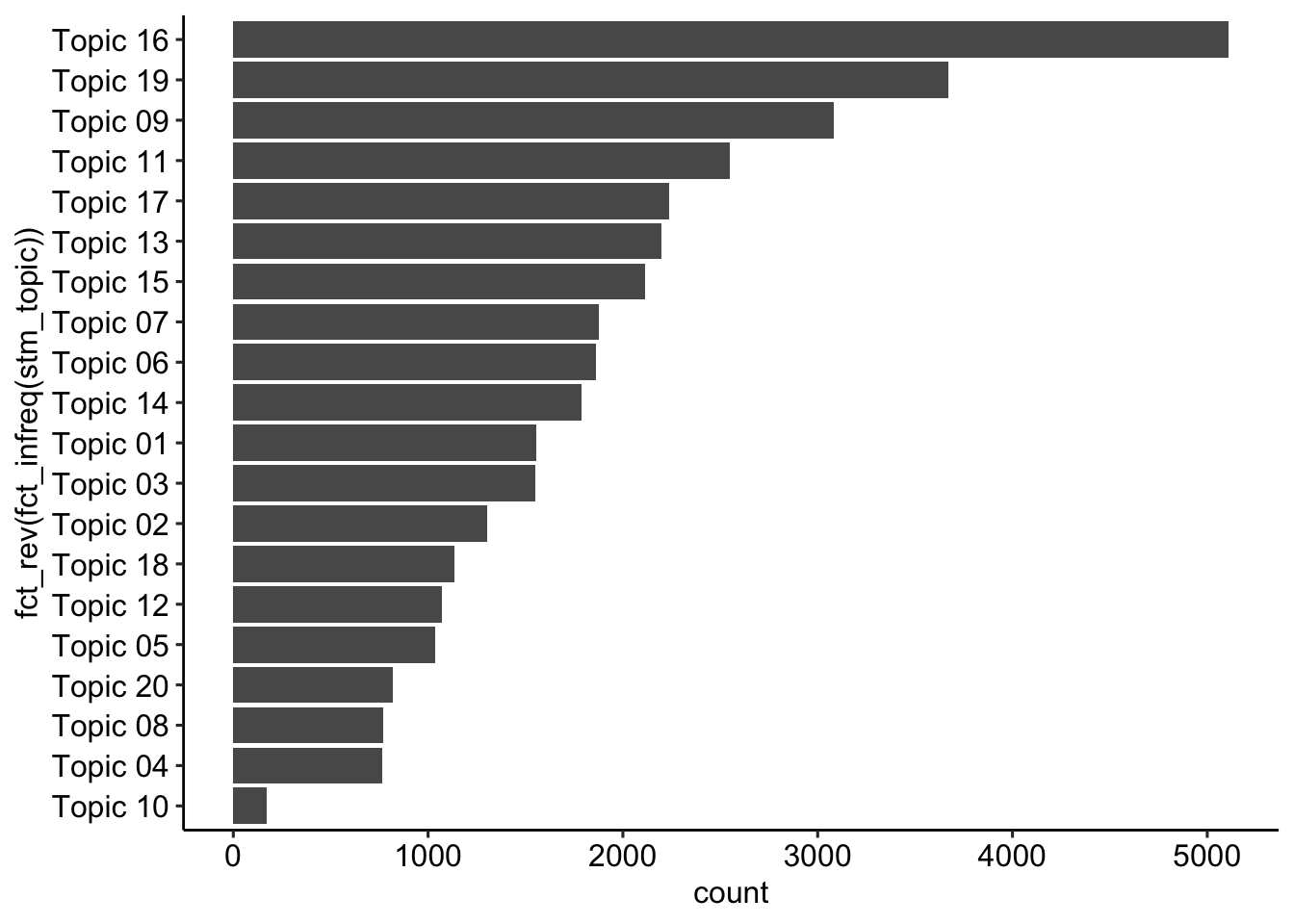

Anzahl der Abstracts nach Thema und Feld

gamma_export %>% 
  gtsummary::tbl_cross(
    row = stm_topic, 
    col = field,
    percent = "row",
    )

	field		Total
	Psychology	Social Sciences	Total
stm_topic
Topic 01	1,470 (94%)	87 (5.6%)	1,557 (100%)
Topic 02	649 (50%)	652 (50%)	1,301 (100%)
Topic 03	1,481 (95%)	71 (4.6%)	1,552 (100%)
Topic 04	459 (60%)	306 (40%)	765 (100%)
Topic 05	301 (29%)	734 (71%)	1,035 (100%)
Topic 06	1,116 (60%)	745 (40%)	1,861 (100%)
Topic 07	825 (44%)	1,051 (56%)	1,876 (100%)
Topic 08	540 (70%)	227 (30%)	767 (100%)
Topic 09	821 (27%)	2,260 (73%)	3,081 (100%)
Topic 10	114 (67%)	57 (33%)	171 (100%)
Topic 11	303 (12%)	2,244 (88%)	2,547 (100%)
Topic 12	439 (41%)	630 (59%)	1,069 (100%)
Topic 13	1,477 (67%)	722 (33%)	2,199 (100%)
Topic 14	509 (28%)	1,277 (72%)	1,786 (100%)
Topic 15	1,815 (86%)	299 (14%)	2,114 (100%)
Topic 16	1,369 (27%)	3,742 (73%)	5,111 (100%)
Topic 17	1,672 (75%)	566 (25%)	2,238 (100%)
Topic 18	737 (65%)	396 (35%)	1,133 (100%)
Topic 19	2,552 (70%)	1,118 (30%)	3,670 (100%)
Topic 20	342 (42%)	475 (58%)	817 (100%)
Total	18,991 (52%)	17,659 (48%)	36,650 (100%)

Fokus: Thema 16

gamma_export %>% 
  filter(stm_topic == "Topic 16") %>%
  arrange(-top_gamma) %>%
  select(title, so, top_gamma, type, ab) %>%
  slice_head(n = 3) %>% 
  gt() %>% 
  fmt_number(
    columns = c(top_gamma), 
    decimals = 2) %>% 
  gtExtras::gt_theme_538()

title	so	top_gamma	type	ab
Theory of Knowledge for Literature Reviews: An Epistemological Model, Taxonomy and Empirical Analysis of IS Literature	NA	0.93	article	Literature reviews play an important role in the development of knowledge. Yet, we observe a lack of theoretical underpinning of and epistemological insights into how literature reviews can contribute to knowledge creation and have actually contributed in the IS discipline. To address these theoretical and empirical research gaps, we suggest a novel epistemological model of literature reviews. This model allows us to align different contributions of literature reviews with their underlying knowledge conversions - thereby building a bridge between the previously largely unconnected fields of literature reviews and epistemology. We evaluate the appropriateness of the model by conducting an empirical analysis of 173 IS literature reviews which were published in 39 pertinent IS journals between 2000 and 2014. Based on this analysis, we derive an epistemological taxonomy of IS literature reviews, which complements previously suggested typologies.
Theory of Knowledge for Literature Reviews: An Epistemological Model, Taxonomy and Empirical Analysis of IS Literature Completed Research Paper	NA	0.93	article	Literature reviews play an important role in the development of knowledge. Yet, we observe a lack of theoretical underpinning of and epistemological insights into how literature reviews can contribute to knowledge creation and have actually contributed in the IS discipline. To address these theoretical and empirical research gaps, we suggest a novel epistemological model of literature reviews. This model allows us to align different contributions of literature reviews with their underlying knowledge conversions - thereby building a bridge between the previously largely unconnected fields of literature reviews and epistemology. We evaluate the appropriateness of the model by conducting an empirical analysis of 173 IS literature reviews which were published in 39 pertinent IS journals between 2000 and 2014. Based on this analysis, we derive an epistemological taxonomy of IS literature reviews, which complements previously suggested typologies.
Relationality in negotiations: a systematic review and propositions for future research	˜The œinternational journal of conflict management/International journal of conflict management	0.93	article	Purpose The purpose of this paper is to systematically review and analyze the important, yet under-researched, topic of relationality in negotiations and propose new directions for future negotiation research. Design/methodology/approach This paper conducts a systematic review of negotiation literature related to relationality from multiple disciplines. Thirty-nine leading and topical academic journals are selected and 574 papers on negotiation are reviewed from 1990 to 2014. Based on the systematic review, propositions regarding the rationales for relationality in negotiations are developed and future research avenues in this area are discussed. Findings Of 574 papers on negotiations published in 39 peer-reviewed journals between 1990 and 2014, only 18 papers have studied and discussed relationality in negotiations. This suggests that relationality as a theoretical theme has long been under-researched in negotiation research. For future research, this paper proposes to incorporate the dynamic, cultural and mechanism perspectives, and to use a qualitative approach to study relationality in negotiations. Originality/value This paper presents the first systematic review of the negotiation literature on relationality, and identifies new research topics on relationality in negotiations. In so doing, this research opens new avenues for future negotiation research on relationality.

Fokus: Thema 6

gamma_export %>% 
  filter(stm_topic == "Topic 06") %>%
  arrange(-top_gamma) %>%
  select(title, so, top_gamma, type, ab) %>%
  slice_head(n = 3) %>% 
  gt() %>% 
  fmt_number(
    columns = c(top_gamma), 
    decimals = 2) %>% 
  gtExtras::gt_theme_538()

title	so	top_gamma	type	ab
The Acceptance of COVID-19 Vaccine: A Global Rapid Systematic Review and Meta-Analysis	Social Science Research Network	0.89	article	Background: Vaccination seems to be the most effective way to prevent and control the spread of COVID-19, a disease that has been playing havoc with the lives of over 7 billion people across the globe. Vaccine hesitancy is probably the most common problem worldwide. This study aims to inspect the COVID-19 vaccine acceptance rates worldwide among the general population and healthcare workers. In addition, it compares the vaccine acceptance rates between the pre-and post-vaccine approval periods.Method: A systematic search was conducted on April 25, 2021, through PubMed, MEDLINE, Web of Science, and GOOGLE SCHOLAR databases using PRISMA and MOOSE statements. Q-test, and statistics were used to search for heterogeneity, and Eggers's test and funnel plot were applied to assess the publication bias. The random-effects model was used to estimate the pooled acceptance rates of the COVID-19 vaccines.Results: The combined COVID-19 vaccine acceptance rate among the general population and healthcare workers (n=1,581,562) was estimated at 61.74%. The vaccine acceptance rate among the general population was 62.66% and the rate among healthcare workers was 57.89%. The acceptance rate decreased from 67.21% to 53.44% among the general population and remained constant among healthcare workers during the pre and post-vaccine approval periods. The acceptance rates also vary in different regions of the world. The highest acceptance rate was found in Western Pacific Region (67.85%) and the lowest was found in African Region (39.51%).Conclusion: Low COVID-19 vaccine acceptance rate might be a massive barrier to getting rid of the pandemic. More researches are needed to address the responsible factors influencing the global rate of COVID-19 vaccine acceptance. Integrated global efforts are required to remove the barriers.
Prevalence of Suicidal Behavior Among Students in South-East Asia: A Systematic Review and Meta-Analysis	Archives of Suicide Research	0.88	article	Estimation of rates of suicidal behaviors (ideation, plan, and attempt) would help to understand the burden and prioritize prevention strategies. However, no attempt to assess suicidal behavior among students was identified in South-East Asia (SEA). We aimed to assess the prevalence of suicidal behavior (ideation, plan, and attempt) among students in SEA.We followed PRISMA 2020 guidelines and registered the protocol in PROSPERO (CRD42022353438). We searched in Medline, Embase, and PsycINFO and performed meta-analyses to pool the lifetime, 1-year, and point prevalence rates for suicidal ideation, plans, and attempts. We considered the duration of a month for point prevalence.The search identified 40 separate populations from which 46 were included in the analyses, as some studies included samples from multiple countries. The pooled prevalence of suicidal ideation was 17.4% (confidence interval [95% CI], 12.4%-23.9%) for lifetime, 9.33% (95% CI, 7.2%-12%) for the past year, and 4.8% (95% CI, 3.6%-6.4%) for the present time. The pooled prevalence of suicide plans was 9% (95% CI, 6.2%-12.9%) for lifetime, 7.3% (95% CI, 5.1%-10.3%) for the past year, and 2.3% (95% CI, 0.8%-6.7%) for the present time. The pooled prevalence of suicide attempts was 5.2% (95% CI, 3.5%-7.8%) for lifetime and 4.5% (95% CI, 3.4%-5.8%) for the past year. Higher rates of suicide attempts in the lifetime were noted in Nepal (10%) and Bangladesh (9%), while lower rates were reported in India (4%) and Indonesia (5%).Suicidal behaviors are a common phenomenon among students in the SEA region. These findings call for integrated, multisectoral efforts to prevent suicidal behaviors in this group.
First COVID-19 Booster Dose in the General Population: A Systematic Review and Meta-Analysis of Willingness and Its Predictors	Vaccines	0.88	article	The emergence of breakthrough infections and new highly contagious variants of SARS-CoV-2 threaten the immunization in individuals who had completed the primary COVID-19 vaccination. This systematic review and meta-analysis investigated, for the first time, acceptance of the first COVID-19 booster dose and its associated factors among fully vaccinated individuals. We followed the PRISMA guidelines. We searched Scopus, Web of Science, Medline, PubMed, ProQuest, CINAHL and medrxiv from inception to 21 May 2022. We found 14 studies including 104,047 fully vaccinated individuals. The prevalence of individuals who intend to accept a booster was 79.0%, while the prevalence of unsure individuals was 12.6%, and the prevalence of individuals that intend to refuse a booster was 14.3%. The main predictors of willingness were older age, flu vaccination in the previous season, and confidence in COVID-19 vaccination. The most important reasons for decline were adverse reactions and discomfort experienced after previous COVID-19 vaccine doses and concerns for serious adverse reactions to COVID-19 booster doses. Considering the burden of COVID-19, a high acceptance rate of booster doses could be critical in controlling the pandemic. Our findings are innovative and could help policymakers to design and implement specific COVID-19 vaccination programs in order to decrease booster vaccine hesitancy.

Die Suche nach dem optimalen k

# Define parameters
future::plan(future::multisession()) # use multiple sessions
topic_range <- seq(from = 10, to = 100, by = 10) 

# Initiate notifications & time tracking
tic("STM extended search")

# Estimate models
stm_search  <- tibble(k = topic_range) %>%
    mutate(
        mdl = furrr::future_map(
            k, 
            ~stm::stm(
                documents = quanteda_stm$documents,
                vocab = quanteda_stm$vocab, 
                prevalence =~ publication_year_fct + field,
                K = ., 
                seed = 42,
                max.em.its = 1000,
                data = quanteda_stm$meta,
                init.type = "Spectral",
                verbose = FALSE),
            .options = furrr::furrr_options(seed = 42)
            )
    )

# Sent status update and finish time tracking
toc(log = TRUE)

Erstellung des “Heldouts”

heldout <- make.heldout(
  documents = quanteda_stm$documents,
  vocab = quanteda_stm$vocab,
  seed = 42)

Evaluation der Modelle

stm_search$results <- stm_search %>%
  mutate(
    exclusivity = map(mdl, exclusivity),
    semantic_coherence = map(mdl, semanticCoherence, quanteda_stm$documents),
    eval_heldout = map(mdl, eval.heldout, heldout$missing),
    residual = map(mdl, checkResiduals, quanteda_stm$documents),
    bound =  map_dbl(mdl, function(x) max(x$convergence$bound)),
    lfact = map_dbl(mdl, function(x) lfactorial(x$settings$dim$K)),
    lbound = bound + lfact,
    iterations = map_dbl(mdl, function(x) length(x$convergence$bound)))

Vergleich verschiedener Statistiken

stm_search$results %>% 
  # Create data for graph
  transmute(
    k, 
    `Lower bound` = lbound,
    Residuals = map_dbl(residual, "dispersion"),
    `Semantic coherence` = map_dbl(semantic_coherence, mean),
    `Held-out likelihood` = map_dbl(eval_heldout, "expected.heldout")
    ) %>%   
  gather(Metric, Value, -k) %>%
  # Create graph
  ggplot(aes(k, Value, color = Metric)) +
    geom_line(linewidth = 1.5, alpha = 0.7, show.legend = FALSE) +
    geom_point(size = 3) +
    # Add marker
    geom_vline(aes(xintercept = 20), color = "#C77CFF", alpha = .5) +
    geom_vline(aes(xintercept = 40), color = "#00BFC4", alpha = .5) +
    geom_vline(aes(xintercept = 60), color = "#C77CFF", alpha = .5) +
    geom_vline(aes(xintercept = 70), color = "#00BFC4", alpha = .5) +  
    scale_x_continuous(breaks = seq(from = 10, to = 100, by = 10)) +
    facet_wrap(~Metric, scales = "free_y") +
    labs(x = "K (number of topics)",
        y = NULL,
        title = "Model diagnostics by number of topics"
        ) +
    theme_pubr()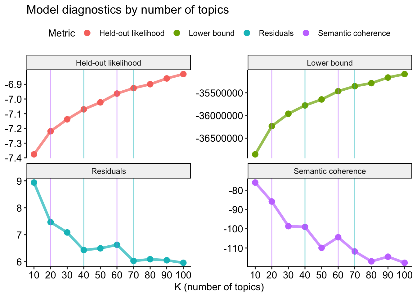

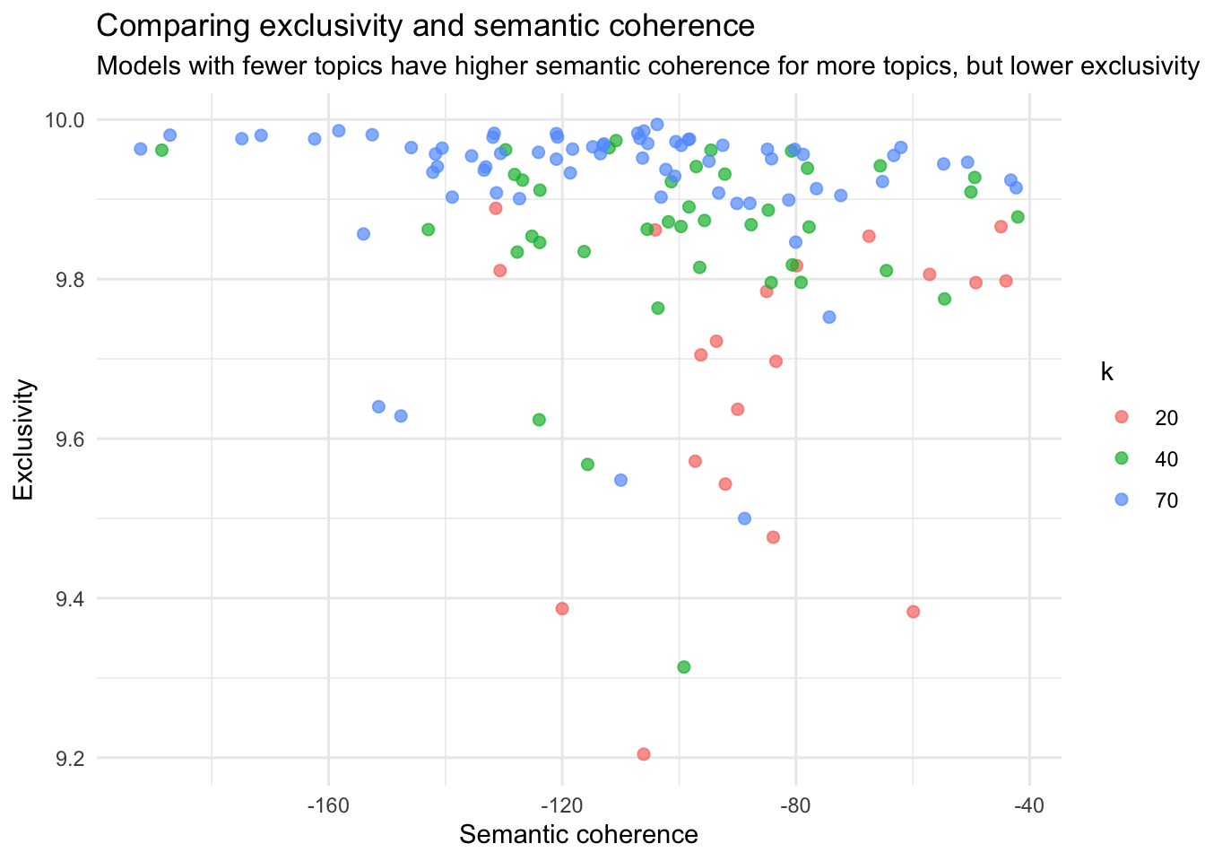
stm_search$results %>% 
  select(k, exclusivity, semantic_coherence) %>% 
  filter(k %in% c(20, 40, 70)) %>%
  unnest(cols = c(exclusivity, semantic_coherence)) %>%
  mutate(k = as.factor(k)) %>%
  ggplot(aes(semantic_coherence, exclusivity, color = k)) +
  geom_point(size = 2, alpha = 0.7) +
  labs(x = "Semantic coherence",
       y = "Exclusivity",
       title = "Comparing exclusivity and semantic coherence",
       subtitle = "Models with fewer topics have higher semantic coherence for more topics, but lower exclusivity"
       ) +
  theme_minimal()