Text processing

Sitzung 08

Christoph Adrian

Chair of Communicaion Science

20.06.2024

Seminarplan

Sitzung	Datum	Thema (synchron)	Übung (asynchron)	Dozent:in
1	18.04.2024	Einführung & Überblick	R-Einführung	AM & CA
2	📚	Teil 1: Systematic Review	R-Einführung	AM
3	25.04.2024	Einführung in Systematic Reviews I	R-Einführung	AM
4	02.05.2024	Einführung in Systematic Reviews II	R-Einführung	AM
5	09.05.2024	🏖️ Feiertag	R-Einführung	ED
6	16.05.2024	Automatisierung von SRs & KI-Tools	R-Einführung	AM
7	23.05.2024	🍻 WiSo-Projekt-Woche	R-Einführung	CA
8	04.06.2024	🍕 Gastvortrag: Prof. Dr. Emese Domahidi	zur Sitzung	CA
9	06.06.2024	Automatisierung von SRs & KI-Tools	zur Sitzung	CA
10	💻	Teil 2: Text as Data & Unsupervised Machine Learning	zur Sitzung	CA & AM
11	13.06.2024	Introduction to Text as Data	zur Sitzung	CA & AM
12	20.06.2024	Text processing	zur Sitzung	CA & AM
1	27.06.2024	Unsupervised Machine Learning I	zur Sitzung	AM & CA
2	04.07.2024	Unsupervised Machine Learning II	R-Einführung	AM
3	11.07.2024	Recap & Ausblick	R-Einführung	AM
4	18.07.2024	🏁 Semesterabschluss	R-Einführung	AM

Agenda

1. Organisation & Koordination

2. From Text to Data

3. Text as data in R

4. 📋 Hands on working with R

Organisation & Koordination

Umorganisation der Kurs-Seite

From Text to Data

Grundbegriffe und Prozess der Texttransformation

Building a shared vocabulary

Wichtige Begriffe und Konzepte

by Analytics Vidhya

Token: A token is a string with a known meaning, and a token may be a word, number or just characters like punctuation. “Hello”, “123”, and “-” are some examples of tokens.

Sentence: A sentence is a group of tokens that is complete in meaning. “The weather looks good” is an example of a sentence, and the tokens of the sentence are [“The”, “weather”, “looks”, “good].

Paragraph: A paragraph is a collection of sentences or phrases, and a sentence can alternatively be viewed as a token of a paragraph.

Documents: A document might be a sentence, a paragraph, or a set of paragraphs. A text message sent to an individual is an example of a document.

Corpus: A corpus is typically an extensive collection of documents as a Bag-of-words. A corpus comprises each word’s id and frequency count in each record. An example of a corpus is a collection of emails or text messages sent to a particular person.

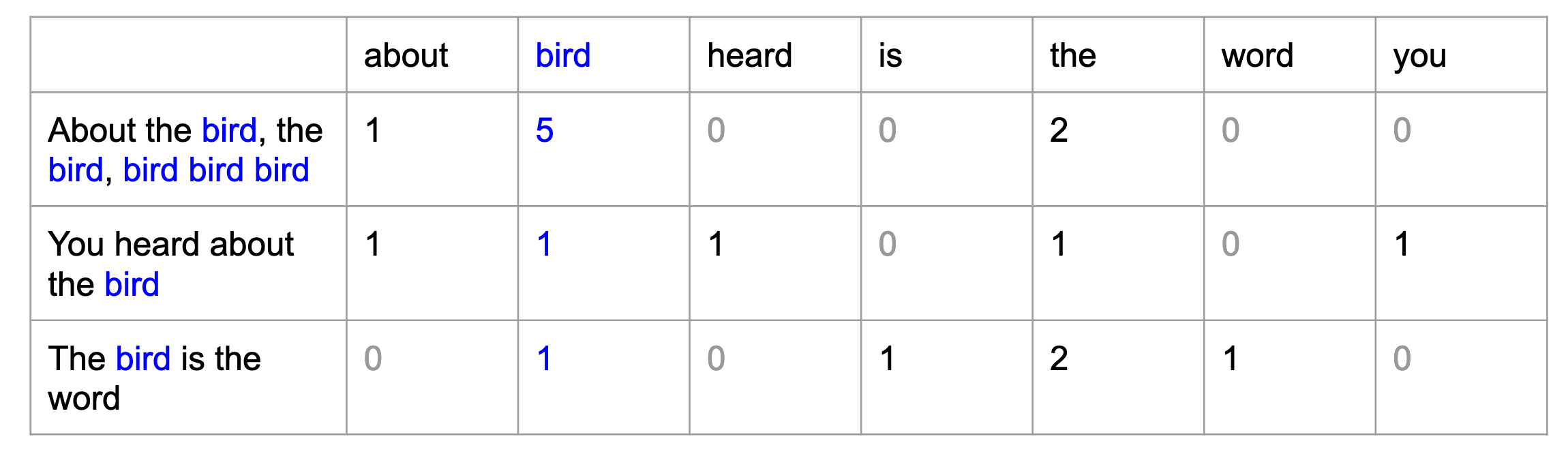
A “bag of words”

Einfache Technik im Natural Language Processing (NLP)

by Shubham Gandhi

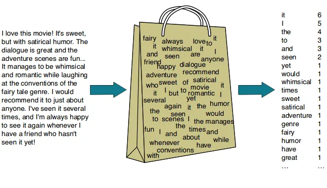
• a collection of words, disregarding grammar, word order, and context.

Digitales Wörterbuch der deutschen Sprache

Großes, frei verfügbares & deutschsprachiges Textkorpora

Vom Korpus zum Token

Einfaches Beispiel zur Darstellung der verschiedenen Konzepte

by Mina Ghashami

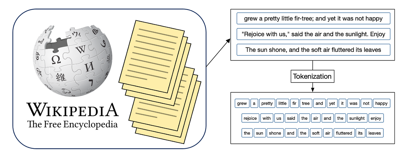
Vom Korpus zum Token zum Model

Komplexer Prozess der Textverarbeitung

by Jiawei Hu

Sätze ➜ Token ➜ Lemma ➜ POS

Beispielhafte Darstellung des Text Preprocessing

1. Satzerkennung

Was gibt’s in New York zu sehen?

2. Tokenisierung

was; gibt; `s; in; new; york; zu; sehen; ?

3. Lemmatisierung

was; geben; `s; in; new; york; zu; sehen; ?

4. Part-Of-Speech (POS) Tagging

>Was/PWS >gibt/VVFIN >’s/PPER >in/APPR >New/NE >York/NE >zu/PTKZU >sehen/VVINF

Satzerkennung: Auflösung der Satzstruktur; Aber: Probleme mit Datumsangaben, Uhrzeit, Abkürzungen, URLS

Tokenisierung: Zerteilung in kleinste Einheiten, Abtrennung von Satzzeichen; Fragen: Umgang mit Zeichen, Symbolen, Zahlen, N-Gramme …

Definition Lemmatisierung: Grundform eines Worters, als diejenige Form, unter dem an einen Begriff in einem Nachschlagewerk findet / Rückführung auf die „Vollfrom”

Definition POS: Zuordnung von Wörtern und Satzzeichen eines Textes zu Wortarten

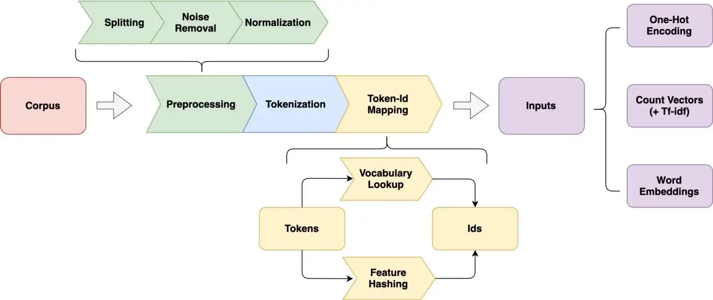
Von BoW zu DFM

Transformation des Bag-of-Words (BOW) zur Document-Feature-Matrix (DFM)

by OpenClassrooms

Bag-of-Words-Modell: es zählt lediglich die Worthäufigkeit je Dokument, die syntaktischen und grammatikalischen Zusammenhänge zwischen einzelnen Wörtern werden ignoriert.

Text as data in R

Einführung in die Textanalyse mit tidytext

What we did so far

Informationen zur Datengrundlage und -quelle

• Suche nach Literatur zur (Sytematischen) Literaturüberblicken auf OpenAlex
• Download von knapp 100.000 Literaturverweisen via API mit openalexR (Aria et al., 2024)
• Deskriptive Auswertung der Daten (“Rekonstruktion” des OpenAlex Web-Dashboards) mit R

Heutige Ziele:

• Eingrenzung der Datenbasis für weiterführende Analysen
• Anwendung einfacher Textanalyseverfahren zur Untersuchung der Abstracts

Euer Input ist gefragt!

Wie sollen die Daten weiter eingegrenzt werden?

Bitte scannt den QR-Code oder nutzt den folgenden Link für die Teilnahme an einer kurzen Umfrage:

• https://www.menti.com/albpi1xur7et

• Temporary Access Code: 3332 2971

01:00

Ergebnis

Build the subsample

Fokus auf englische Artikel aus den Sozialwissenschaften und der Psychologie

review_subsample <- review_works_correct %>% 
  # Eingrenzung: Sprache und Typ
  filter(language == "en") %>% 
  filter(type == "article") %>%
  # Datentranformation
  unnest(topics, names_sep = "_") %>%
  filter(topics_name == "field") %>% 
  filter(topics_i == "1") %>% 
  # Eingrenzung: Forschungsfeldes
  filter(
   topics_display_name == "Social Sciences"|
   topics_display_name == "Psychology"
    )

review_works_correct %>% 
  mutate(
    included = ifelse(id %in% review_subsample$id, "Ja", "Nein"),
    included = factor(included, levels = c("Nein", "Ja"))
    ) %>%
  ggplot(aes(x = publication_year_fct, fill = included)) +
    geom_bar() +
    labs(
      x = "",
      y = "Anzahl der Einträge", 
      fill = "In Subsample enthalten?"
     ) +
    scale_fill_manual(values = c("#A0ACBD50", "#FF707F")) +
    theme_pubr()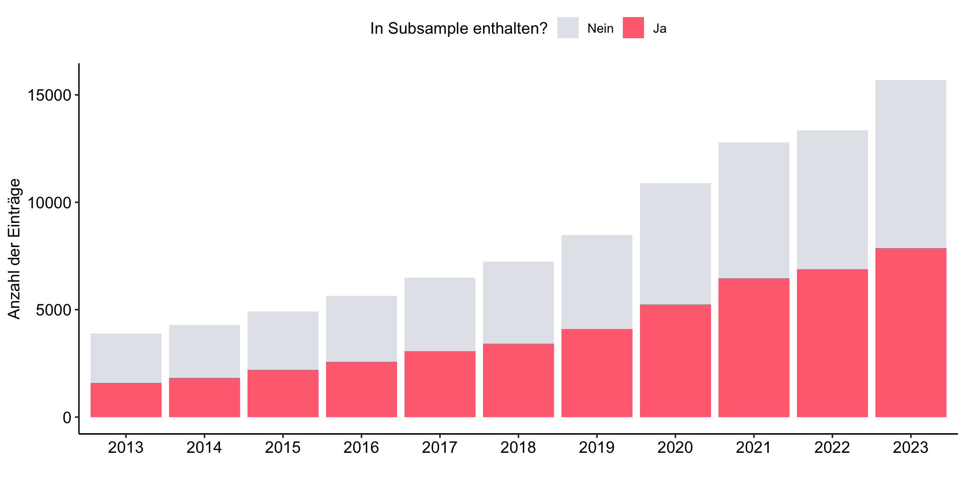 

Explore abstracts

Tidy data principles als Grundlage für Analyse-Workflow

(Silge & Robinson, 2017)

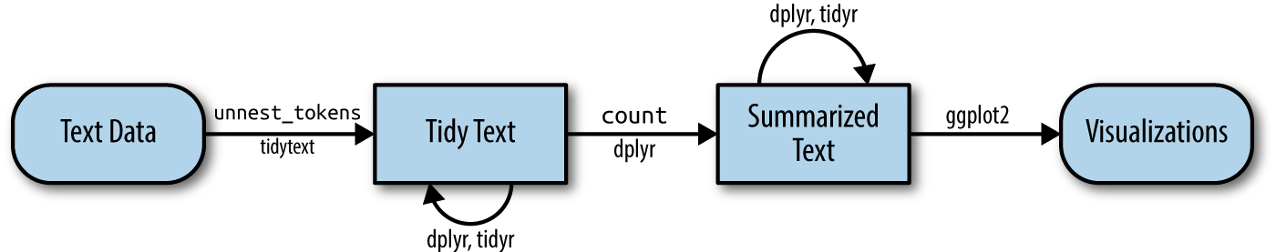
• Tidy data struture (each variable is column, each observation a row, each value is a cell, each type of observaional unit is a table) results in a table with one-token-per-row (Silge & Robinson, 2017).

Tokenization der Abstracts

Transform data to tidy text

# Create tidy data
review_tidy <- review_subsample %>% 
    # Tokenization
    tidytext::unnest_tokens("text", ab) %>% 
    # Remove stopwords
    filter(!text %in% tidytext::stop_words$word)

# Preview
review_tidy %>% 
  select(id, text) %>% 
  print(n = 10)

# A tibble: 4,880,965 × 2
   id                               text          
   <chr>                            <chr>         
 1 https://openalex.org/W4293003987 5             
 2 https://openalex.org/W4293003987 item          
 3 https://openalex.org/W4293003987 world         
 4 https://openalex.org/W4293003987 health        
 5 https://openalex.org/W4293003987 organization  
 6 https://openalex.org/W4293003987 index         
 7 https://openalex.org/W4293003987 5             
 8 https://openalex.org/W4293003987 widely        
 9 https://openalex.org/W4293003987 questionnaires
10 https://openalex.org/W4293003987 assessing     
# ℹ 4,880,955 more rows

Before and after the transformation

Vergleich eines Abstraktes in Rohform und nach Tokenisierung

review_subsample$ab[[1]]

[1] "The 5-item World Health Organization Well-Being Index (WHO-5) is among the most widely used questionnaires assessing subjective psychological well-being. Since its first publication in 1998, the WHO-5 has been translated into more than 30 languages and has been used in research studies all over the world. We now provide a systematic review of the literature on the WHO-5.We conducted a systematic search for literature on the WHO-5 in PubMed and PsycINFO in accordance with the PRISMA guidelines. In our review of the identified articles, we focused particularly on the following aspects: (1) the clinimetric validity of the WHO-5; (2) the responsiveness/sensitivity of the WHO-5 in controlled clinical trials; (3) the potential of the WHO-5 as a screening tool for depression, and (4) the applicability of the WHO-5 across study fields.A total of 213 articles met the predefined criteria for inclusion in the review. The review demonstrated that the WHO-5 has high clinimetric validity, can be used as an outcome measure balancing the wanted and unwanted effects of treatments, is a sensitive and specific screening tool for depression and its applicability across study fields is very high.The WHO-5 is a short questionnaire consisting of 5 simple and non-invasive questions, which tap into the subjective well-being of the respondents. The scale has adequate validity both as a screening tool for depression and as an outcome measure in clinical trials and has been applied successfully across a wide range of study fields."

review_tidy %>% 
  filter(id == "https://openalex.org/W4293003987") %>% 
  pull(text) %>% 
  paste(collapse = " ")

[1] "5 item world health organization index 5 widely questionnaires assessing subjective psychological publication 1998 5 translated 30 languages research studies world provide systematic review literature 5 conducted systematic search literature 5 pubmed psycinfo accordance prisma guidelines review identified articles focused aspects 1 clinimetric validity 5 2 responsiveness sensitivity 5 controlled clinical trials 3 potential 5 screening tool depression 4 applicability 5 study fields.a total 213 articles met predefined criteria inclusion review review demonstrated 5 clinimetric validity outcome measure balancing unwanted effects treatments sensitive specific screening tool depression applicability study fields high.the 5 short questionnaire consisting 5 simple invasive questions tap subjective respondents scale adequate validity screening tool depression outcome measure clinical trials applied successfully wide range study fields"

Count token frequency

Summarize all tokens over all tweets

# Create summarized data
review_summarized <- review_tidy %>% 
  count(text, sort = TRUE) 

# Preview Top 15 token
review_summarized %>% 
    print(n = 15)

# A tibble: 122,148 × 2
   text              n
   <chr>         <int>
 1 studies       73398
 2 review        57878
 3 research      42689
 4 health        35108
 5 systematic    32431
 6 literature    31374
 7 study         29012
 8 interventions 22731
 9 included      21987
10 social        21528
11 articles      20631
12 results       20166
13 analysis      19624
14 based         18929
15 evidence      18545
# ℹ 122,133 more rows

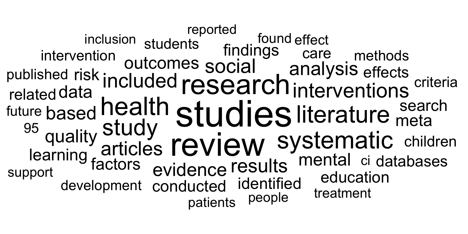
The (Unavoidable) Word Cloud

Visualization of Top 50 token

review_summarized %>% 
    top_n(50) %>% 
    ggplot(aes(label = text, size = n)) +
    ggwordcloud::geom_text_wordcloud() +
    scale_size_area(max_size = 20) +
    theme_minimal()

Mehr als nur ein Wort

Modellierung von Wortzusammenhängen: n-grams and correlations

Viele der wirklich interessanten Ergebnisse von Textanalysen basieren auf den Beziehungen zwischen Wörtern, z.B.

• welche Wörter dazu “neigen”, unmittelbar auf einander zu folgen (n-grams),
• oder innerhalb desselben Dokuments gemeinsam aufzutreten (Korrelation)

(Silge & Robinson, 2017)

Häufige Wortpaare

Wortkombinationen (n-grams) im FokusH

# Create word paris
review_word_pairs <- review_tidy %>% 
    widyr::pairwise_count(
        text,
        id,
        sort = TRUE)

# Preview
review_word_pairs %>% 
    print(n = 14)

# A tibble: 114,446,724 × 3
   item1      item2          n
   <chr>      <chr>      <dbl>
 1 review     studies    20494
 2 studies    review     20494
 3 review     systematic 20266
 4 systematic review     20266
 5 review     research   16902
 6 research   review     16902
 7 literature review     16754
 8 review     literature 16754
 9 systematic studies    16097
10 studies    systematic 16097
11 study      review     13391
12 review     study      13391
13 studies    research   13173
14 research   studies    13173
# ℹ 114,446,710 more rows

Häufig zusammen, selten allein

Wortkorrelationen im Fokus

# Create word correlation
review_pairs_corr <- review_tidy %>% 
    group_by(text) %>% 
    filter(n() >= 300) %>% 
    pairwise_cor(
        text, 
        id, 
        sort = TRUE)

# Preview
review_pairs_corr %>% 
    print(n = 15)

# A tibble: 5,529,552 × 3
   item1      item2      correlation
   <chr>      <chr>            <dbl>
 1 ottawa     newcastle        0.977
 2 newcastle  ottawa           0.977
 3 briggs     joanna           0.967
 4 joanna     briggs           0.967
 5 scholar    google           0.938
 6 google     scholar          0.938
 7 obsessive  compulsive       0.929
 8 compulsive obsessive        0.929
 9 nervosa    anorexia         0.893
10 anorexia   nervosa          0.893
11 ci         95               0.887
12 95         ci               0.887
13 las        los              0.886
14 los        las              0.886
15 gay        bisexual         0.861
# ℹ 5,529,537 more rows

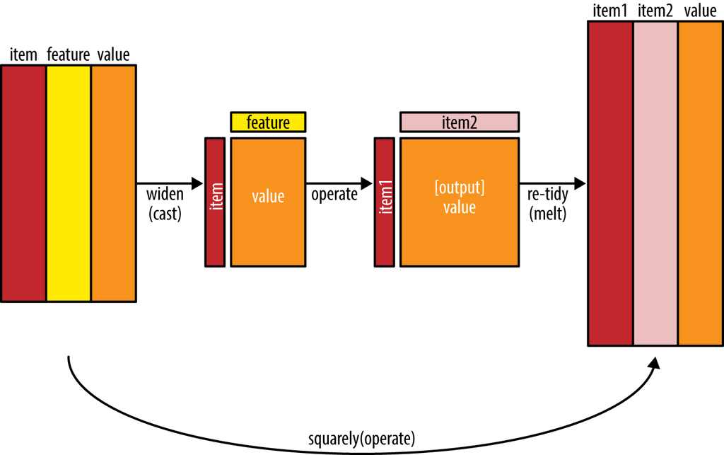
Spezifische “Partner” in spezifischen Umgebungen

Häufig auftretenden Wörter in der Umgebung von review, literature, systematic

review_pairs_corr %>% 
  filter(
    item1 %in% c(
      "review",
      "literature",
      "systematic")
    ) %>% 
  group_by(item1) %>% 
  slice_max(correlation, n = 5) %>% 
  ungroup() %>% 
  mutate(
    item2 = reorder(item2, correlation)
    ) %>% 
  ggplot(
    aes(item2, correlation, fill = item1)
    ) +
  geom_bar(stat = "identity") +
  facet_wrap(~ item1, scales = "free_y") +
  coord_flip() +
  scale_fill_manual(
    values = c(
      "#04316A",
      "#C50F3C",
      "#00B2D1")) +
  theme_pubr()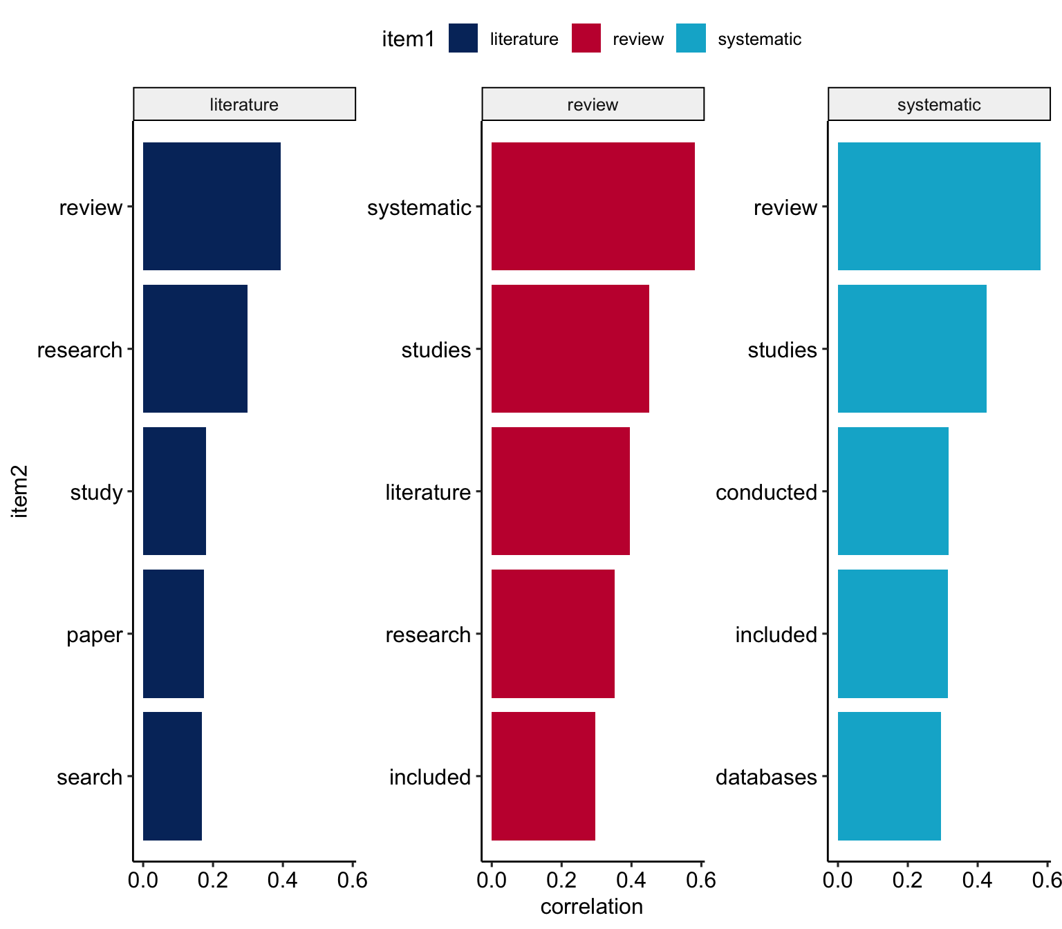

Let’s talk about sentiments

Dictionary based approach of text analysis

(Silge & Robinson, 2017)

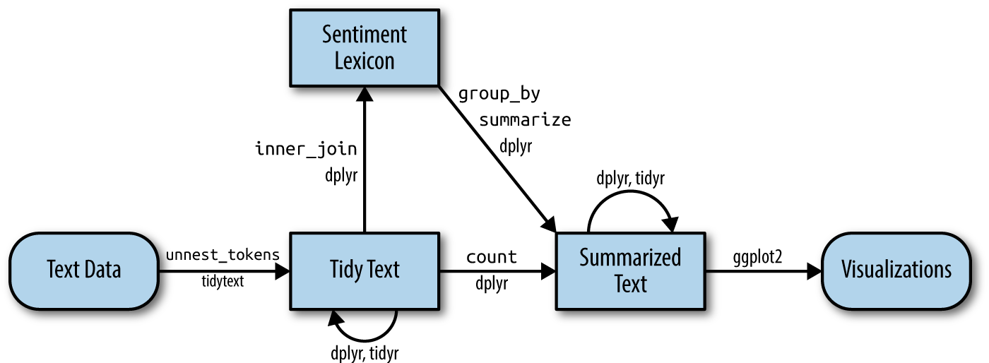
Atteveldt et al. (2021) argue that sentiment, in fact, are quite a complex concepts that are often hard to capture with dictionaries.

Über die Bedeutung von “positiv;negativ”

Die häufigsten “positiven” und “negativen” Wörter in den Abstracts

review_sentiment_count <- review_tidy %>% 
  inner_join(
     get_sentiments("bing"),
     by = c("text" = "word"),
     relationship = "many-to-many") %>% 
  count(text, sentiment)
  
# Preview
review_sentiment_count %>% 
  group_by(sentiment) %>%
  slice_max(n, n = 10) %>% 
  ungroup() %>% 
  mutate(text = reorder(text, n)) %>%
  ggplot(aes(n, text, fill = sentiment)) +
  geom_col(show.legend = FALSE) +
  facet_wrap(
    ~sentiment, scales = "free_y") +
  labs(x = "Contribution to sentiment",
       y = NULL) +
  scale_fill_manual(
    values = c("#C50F3C", "#007900")) +
  theme_pubr()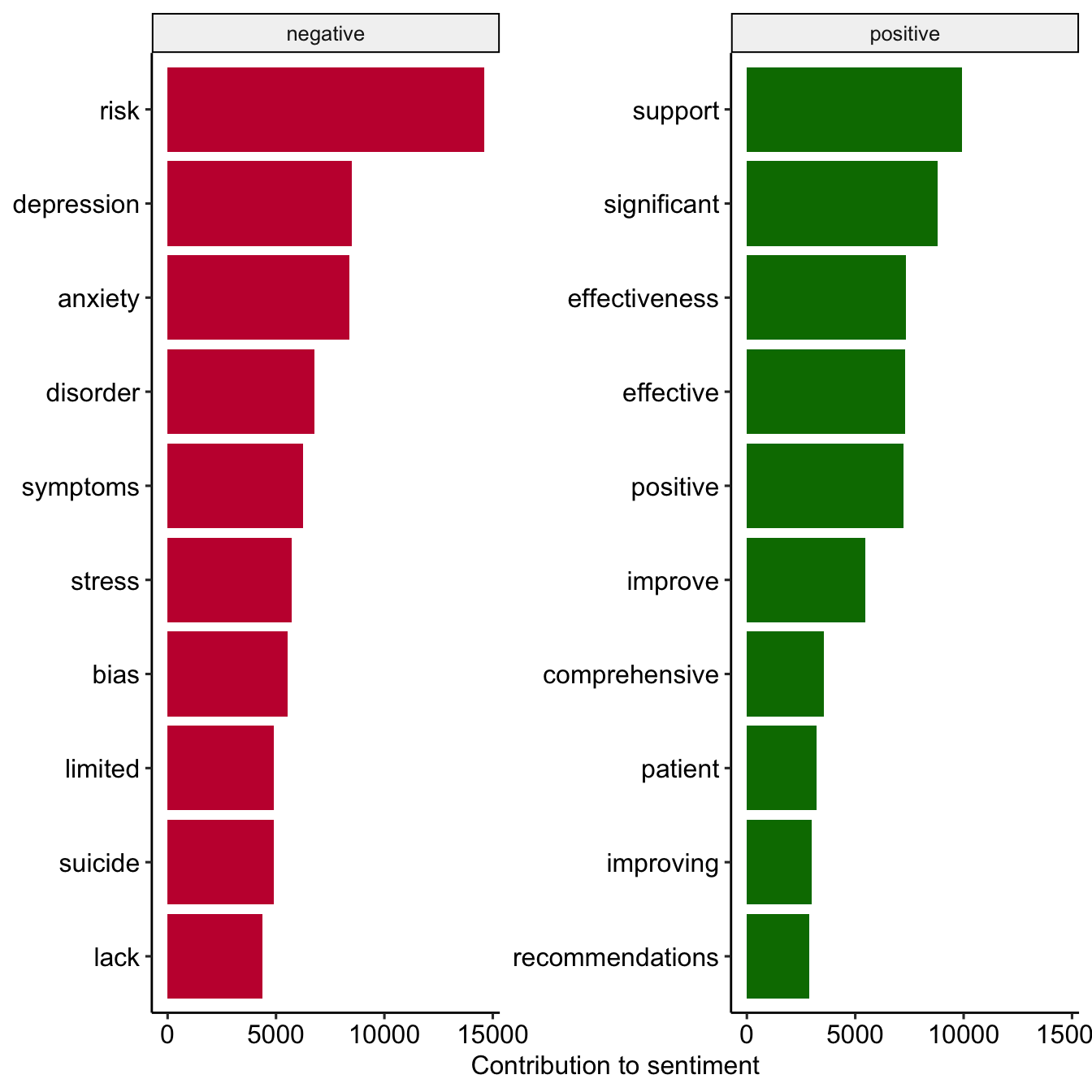

Anreicherung der Daten

Verknüpfung des Sentiemnt (Scores) mit den Abstracts

review_sentiment <- review_tidy %>% 
  inner_join(
     get_sentiments("bing"),
     by = c("text" = "word"),
     relationship = "many-to-many") %>% 
  count(id, sentiment) %>% 
  pivot_wider(names_from = sentiment, values_from = n, values_fill = 0) %>% 
  mutate(sentiment = positive - negative)
  
# Check
review_sentiment 

# A tibble: 35,710 × 4
   id                               negative positive sentiment
   <chr>                               <int>    <int>     <int>
 1 https://openalex.org/W1000529773        2        2         0
 2 https://openalex.org/W1006561082        0        1         1
 3 https://openalex.org/W100685805         4       15        11
 4 https://openalex.org/W1007410967        0        7         7
 5 https://openalex.org/W1008209175        8        1        -7
 6 https://openalex.org/W1009104829        2        4         2
 7 https://openalex.org/W1009607471       15        8        -7
 8 https://openalex.org/W1031503832       13        6        -7
 9 https://openalex.org/W1035654938       10        5        -5
10 https://openalex.org/W1044055445        5        0        -5
# ℹ 35,700 more rows

Neutral, mit einem leicht “negativen” Unterton

Verteilung des Sentiment (Scores) in den Abstracts

[1] 0.4858737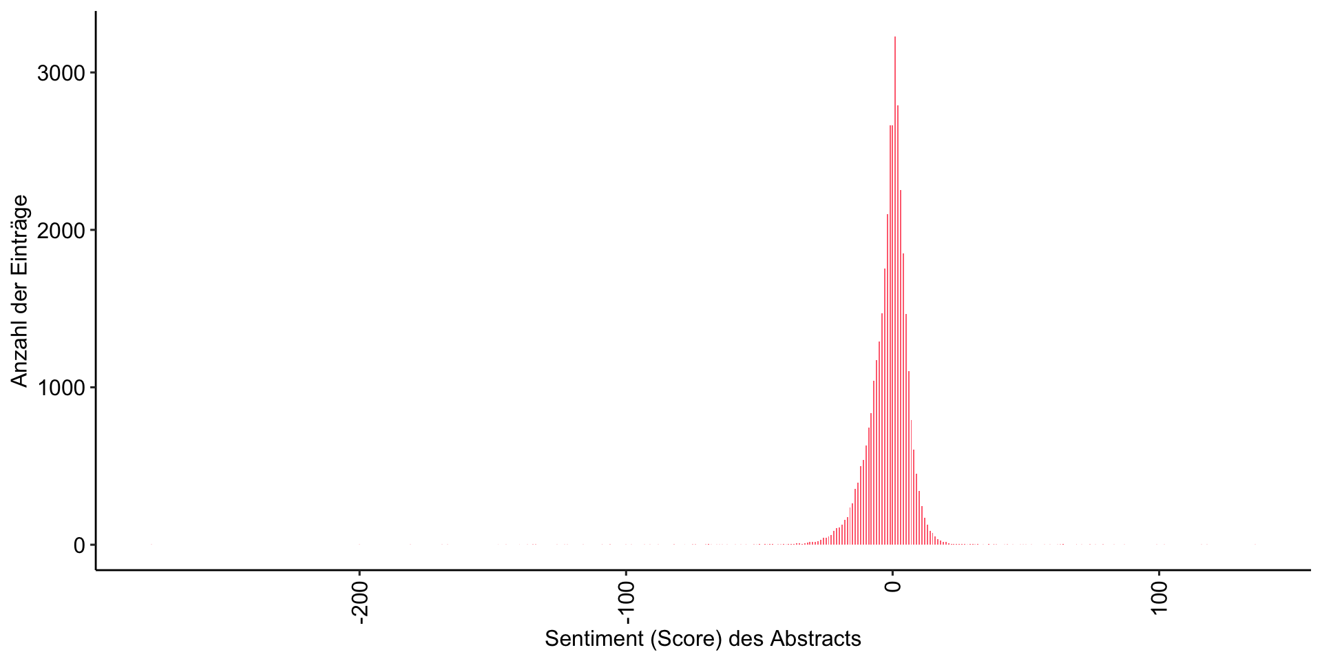

review_sentiment %>% 
  ggplot(aes(sentiment)) +
  geom_histogram(binwidth = 0.5, fill = "#FF707F") +
  labs(
    x = "Sentiment (Score) des Abstracts", 
    y = "Anzahl der Einträge"
  ) +
  theme_pubr() +
  theme(axis.text.x = element_text(angle = 90, vjust = 0.5, hjust=1))

Keep it neutral

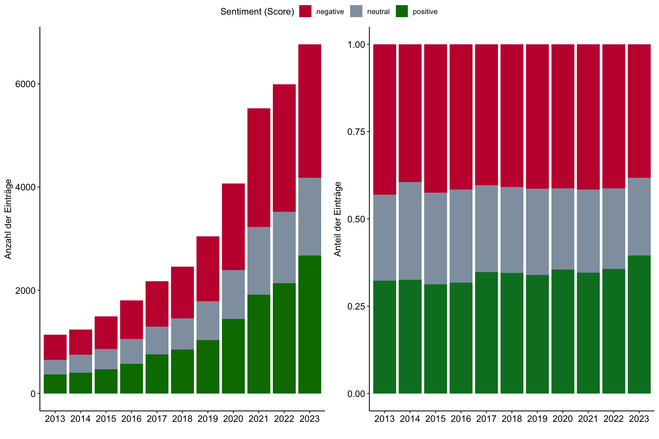
Entwicklung des Sentiment (Scores) der Abstracts im Zeitverlauf

# Create first graph
g1 <- review_works_correct %>% 
  filter(id %in% review_sentiment$id) %>% 
  left_join(review_sentiment, by = join_by(id)) %>% 
  sjmisc::rec(
    sentiment,
    rec = "min:-2=negative; -1:1=neutral; 2:max=positive") %>% 
  ggplot(aes(x = publication_year_fct, fill = as.factor(sentiment_r))) +
    geom_bar() +
    labs(
      x = "",
      y = "Anzahl der Einträge", 
      fill = "Sentiment (Score)") +
    scale_fill_manual(values = c("#C50F3C", "#90A0AF", "#007900")) +
    theme_pubr() 
    #theme(axis.text.x = element_text(angle = 90, vjust = 0.5, hjust=1))

# Create second graph
g2 <- review_works_correct %>% 
  filter(id %in% review_sentiment$id) %>% 
  left_join(review_sentiment, by = join_by(id)) %>% 
  sjmisc::rec(
    sentiment,
    rec = "min:-2=negative; -1:1=neutral; 2:max=positive") %>% 
  ggplot(aes(x = publication_year_fct, fill = as.factor(sentiment_r))) +
    geom_bar(position = "fill") +
    labs(
      x = "",
      y = "Anteil der Einträge", 
      fill = "Sentiment (Score)") +
    scale_fill_manual(values = c("#C50F3C", "#90A0AF", "#007D29")) +
    theme_pubr() 

# COMBINE GRPAHS
ggarrange(g1, g2,
          nrow = 1, ncol = 2, 
          align = "hv",
          common.legend = TRUE) 

📋 Hands on working with R

Verschiedene R-Übungsaufgaben zum Inhalt der heutigen Sitzung

🧪 And now … you: Wiederholung

Next Steps: Wiederholung der R-Grundlagen an OpenAlex-Daten

• Laden Sie die auf StudOn bereitgestellten Dateien für die Sitzungen herunter
• Laden Sie die .zip-Datei in Ihren RStudio Workspace
• Navigieren Sie zu dem Ordner, in dem die Datei ps_24_binder.Rproj liegt. Öffnen Sie diese Datei mit einem Doppelklick. Nur dadurch ist gewährleistet, dass alle Dependencies korrekt funktionieren.
• Öffnen Sie die Datei exercise-08.qmd im Ordner exercises und lesen Sie sich gründlich die Anweisungen durch.
• Tipp: Sie finden alle in den Folien verwendeten Code-Bausteine in der Datei showcase.qmd (für den “rohen” Code) oder showcase.html (mit gerenderten Ausgaben).

Time for questions

Danke & bis zur nächsten Sitzung!

Literatur

Aria, M., Le, T., Cuccurullo, C., Belfiore, A., & Choe, J. (2024). openalexR: An R-Tool for Collecting Bibliometric Data from OpenAlex. The R Journal, 15(4), 167–180. https://doi.org/10.32614/rj-2023-089

Atteveldt, W. van, Trilling, D., & Arcíla, C. (2021). Computational analysis of communication: A practical introduction to the analysis of texts, networks, and images with code examples in python and r. John Wiley & Sons.

Silge, J., & Robinson, D. (2017). Text mining with r: A tidy approach (First edition). O’Reilly.