pacman::p_load(
  here,
  magrittr,
  tidyverse,
  janitor,
  easystats,
  sjmisc,
ggpubr)Exercise 03: 🔨 Working with R
Hollywood Age Gap
![]() Download source file
Download source file
![]() Open this exercise in interactive and executable environment
Open this exercise in interactive and executable environment
Background
- The best way to learn R is by trying. This document tries to display a version of the “normal” data processing procedure.
- Use
tidytuesdaydata as an example to showcase the potential
Todays’s data basis: Hollywood Age Gaps
An informational site showing the age gap between movie love interests.
The data follows certain rules:
- The two (or more) actors play actual love interests (not just friends, coworkers, or some other non-romantic type of relationship)
- The youngest of the two actors is at least 17 years old
- Not animated characters
Packages
Zum Laden der Pakete wird das Paket
pacman::pload()genutzt, dass gegenüber der herkömmlichen Methode mitlibrary()eine Reihe an Vorteile hat:- Prägnante Syntax
- Automatische Installation (wenn Paket noch nicht vorhanden)
- Laden mehrerer Pakete auf einmal
- Automatische Suche nach
dependencies
Codechunks aus der Sitzung
Die erste “Runde” der Datenaufbereitung
Datenimport via URL
| Variable | Description |
|---|---|
movie_name |
Name of the film |
release_year |
Release year |
director |
Director of the film |
age_difference |
Age difference between the characters in whole years |
couple_number |
An identifier for the couple in case multiple couples are listed for this film |
actor_1_name |
The name of the older actor in this couple |
actor_2_name |
The name of the younger actor in this couple |
actor_1_birthdate |
The birthdate of the older member of the couple |
actor_2_birthdate |
The birthdate of the younger member of the couple |
actor_1_age |
The age of the older actor when the film was released |
actor_2_age |
The age of the younger actor when the film was released |
# Import data from URL
age_gaps <- read_csv("http://hollywoodagegap.com/movies.csv") %>%
  janitor::clean_names()

# Check data set
age_gaps
# A tibble: 1,177 × 12
movie_name release_year director age_difference actor_1_name actor_1_gender
<chr> <dbl> <chr> <dbl> <chr> <chr>
1 Harold and … 1971 Hal Ash… 52 Bud Cort man
2 Venus 2006 Roger M… 50 Peter O'Too… man
3 The Quiet A… 2002 Phillip… 49 Michael Cai… man
4 The Big Leb… 1998 Joel Co… 45 David Huddl… man
5 Beginners 2010 Mike Mi… 43 Christopher… man
6 Poison Ivy 1992 Katt Sh… 42 Tom Skerritt man
7 Whatever Wo… 2009 Woody A… 40 Larry David man
8 Entrapment 1999 Jon Ami… 39 Sean Connery man
9 Husbands an… 1992 Woody A… 38 Woody Allen man
10 Magnolia 1999 Paul Th… 38 Jason Robar… man
# ℹ 1,167 more rows
# ℹ 6 more variables: actor_1_birthdate <date>, actor_1_age <dbl>,
# actor_2_name <chr>, actor_2_gender <chr>, actor_2_birthdate <chr>,
# actor_2_age <dbl>Initiale Überprüfung der Daten
Sind die Daten “technisch korrekt”?
Überblick über die Daten
age_gaps %>% glimpse()Rows: 1,177
Columns: 12
$ movie_name <chr> "Harold and Maude", "Venus", "The Quiet American", "…
$ release_year <dbl> 1971, 2006, 2002, 1998, 2010, 1992, 2009, 1999, 1992…
$ director <chr> "Hal Ashby", "Roger Michell", "Phillip Noyce", "Joel…
$ age_difference <dbl> 52, 50, 49, 45, 43, 42, 40, 39, 38, 38, 36, 36, 35, …
$ actor_1_name <chr> "Bud Cort", "Peter O'Toole", "Michael Caine", "David…
$ actor_1_gender <chr> "man", "man", "man", "man", "man", "man", "man", "ma…
$ actor_1_birthdate <date> 1948-03-29, 1932-08-02, 1933-03-14, 1930-09-17, 192…
$ actor_1_age <dbl> 23, 74, 69, 68, 81, 59, 62, 69, 57, 77, 59, 56, 65, …
$ actor_2_name <chr> "Ruth Gordon", "Jodie Whittaker", "Do Thi Hai Yen", …
$ actor_2_gender <chr> "woman", "woman", "woman", "woman", "man", "woman", …
$ actor_2_birthdate <chr> "1896-10-30", "1982-06-03", "1982-10-01", "1975-11-0…
$ actor_2_age <dbl> 75, 24, 20, 23, 38, 17, 22, 30, 19, 39, 23, 20, 30, …Korrekturen
age_gaps_correct <- age_gaps %>%
  mutate(
    across(ends_with("_birthdate"), ~as.Date(.)) # set dates to dates
  )
Überprüfung Lageparameter
age_gaps_correct %>% descr()
## Basic descriptive statistics

            var    type          label    n NA.prc    mean    sd   se   md
   release_year numeric   release_year 1177      0 2000.74 16.67 0.49 2004
 age_difference numeric age_difference 1177      0   10.48  8.53 0.25    8
    actor_1_age numeric    actor_1_age 1177      0   39.97 10.90 0.32   39
    actor_2_age numeric    actor_2_age 1177      0   31.27  8.50 0.25   30
 trimmed          range iqr  skew
 2003.65 88 (1935-2023)  15 -1.68
    9.41      52 (0-52)  12  1.19
   39.41     64 (17-81)  15  0.53
   30.42     64 (17-81)   9  1.39
Die ersten Datenexplorationen
Wie sind die Altersunterschiede verteilt?
age_gaps_correct %>%
    ggplot(aes(x = age_difference)) +
    geom_bar() +
    theme_pubr()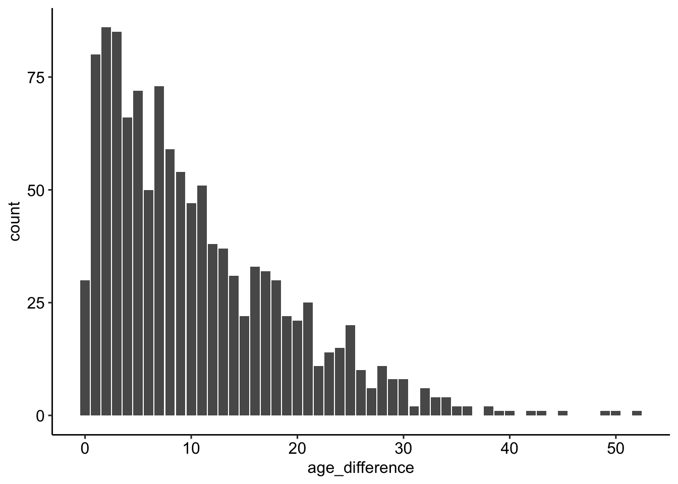
In welchen Filmen ist der Altersunterschied am höchsten?
age_gaps_correct %>%
    arrange(desc(age_difference)) %>%
    select(movie_name, age_difference, release_year)
# A tibble: 1,177 × 3
movie_name age_difference release_year
<chr> <dbl> <dbl>
1 Harold and Maude 52 1971
2 Venus 50 2006
3 The Quiet American 49 2002
4 The Big Lebowski 45 1998
5 Beginners 43 2010
6 Poison Ivy 42 1992
7 Whatever Works 40 2009
8 Entrapment 39 1999
9 Husbands and Wives 38 1992
10 Magnolia 38 1999
# ℹ 1,167 more rowsage_gaps_correct %>%
filter(release_year >= 2022) %>%
arrange(desc(age_difference)) %>%
select(
movie_name, age_difference, release_year,
actor_1_name, actor_2_name) # A tibble: 12 × 5
movie_name age_difference release_year actor_1_name actor_2_name
<chr> <dbl> <dbl> <chr> <chr>
1 The Bubble 21 2022 Pedro Pascal Maria Bakal…
2 Oppenheimer 20 2023 Cillian Mur… Florence Pu…
3 The Northman 20 2022 Alexander S… Anya Taylor…
4 The Lost City 16 2022 Channing Ta… Sandra Bull…
5 Barbie 10 2023 Ryan Gosling Margot Robb…
6 Everything Everywhere … 9 2022 Ke Huy Quan Michelle Ye…
7 Top Gun: Maverick 8 2022 Tom Cruise Jennifer Co…
8 Oppenheimer 7 2023 Cillian Mur… Emily Blunt
9 Your Place or Mine 7 2023 Ashton Kutc… Zoë Chao
10 Your Place or Mine 5 2023 Jesse Willi… Reese Withe…
11 Your Place or Mine 2 2023 Ashton Kutc… Reese Withe…
12 You People 1 2023 Jonah Hill Lauren Lond…Gibt es einen Zusammenhang zwischen Altersunterschied und Release?
(Durchschnitts-)Unterschied nach Jahren
age_gaps_correct %>%
    group_by(release_year) %>%
    summarise(age_difference_mean = mean(age_difference)) %>%
    ggplot(aes(release_year, age_difference_mean)) +
    geom_col() +
    theme_pubr()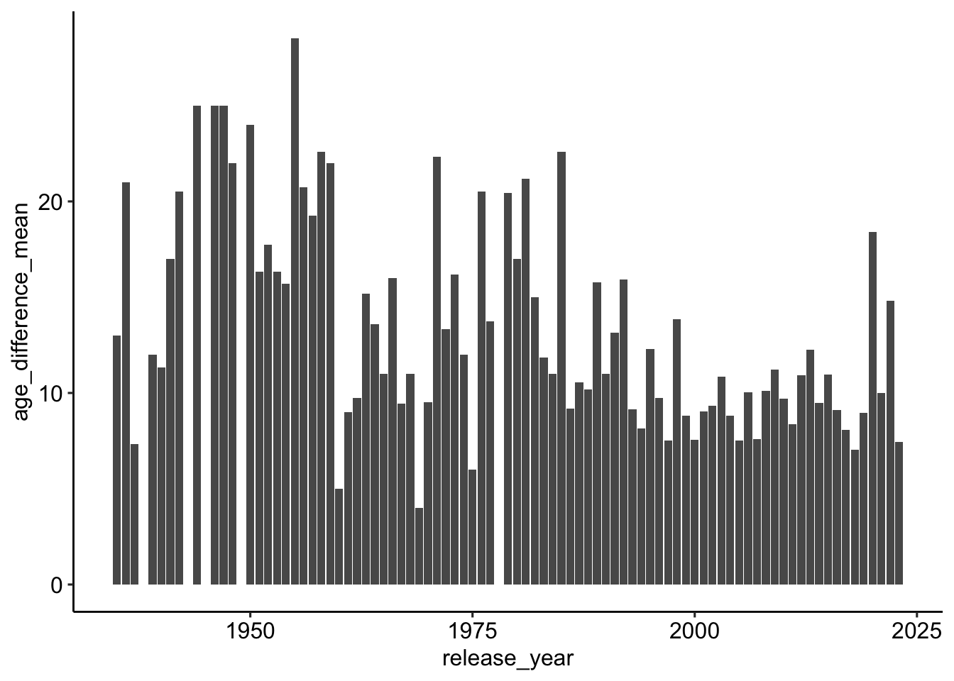
Verteilung nach Jahren
ggpubr::ggboxplot(
    data = age_gaps_correct,
    x = "release_year",
    y = "age_difference",
  ) +
   # Rotate x-axis labels by 90 degrees
  theme(
    axis.text.x = element_text(
        angle = 90,
        vjust = 0.5,
hjust=1)) 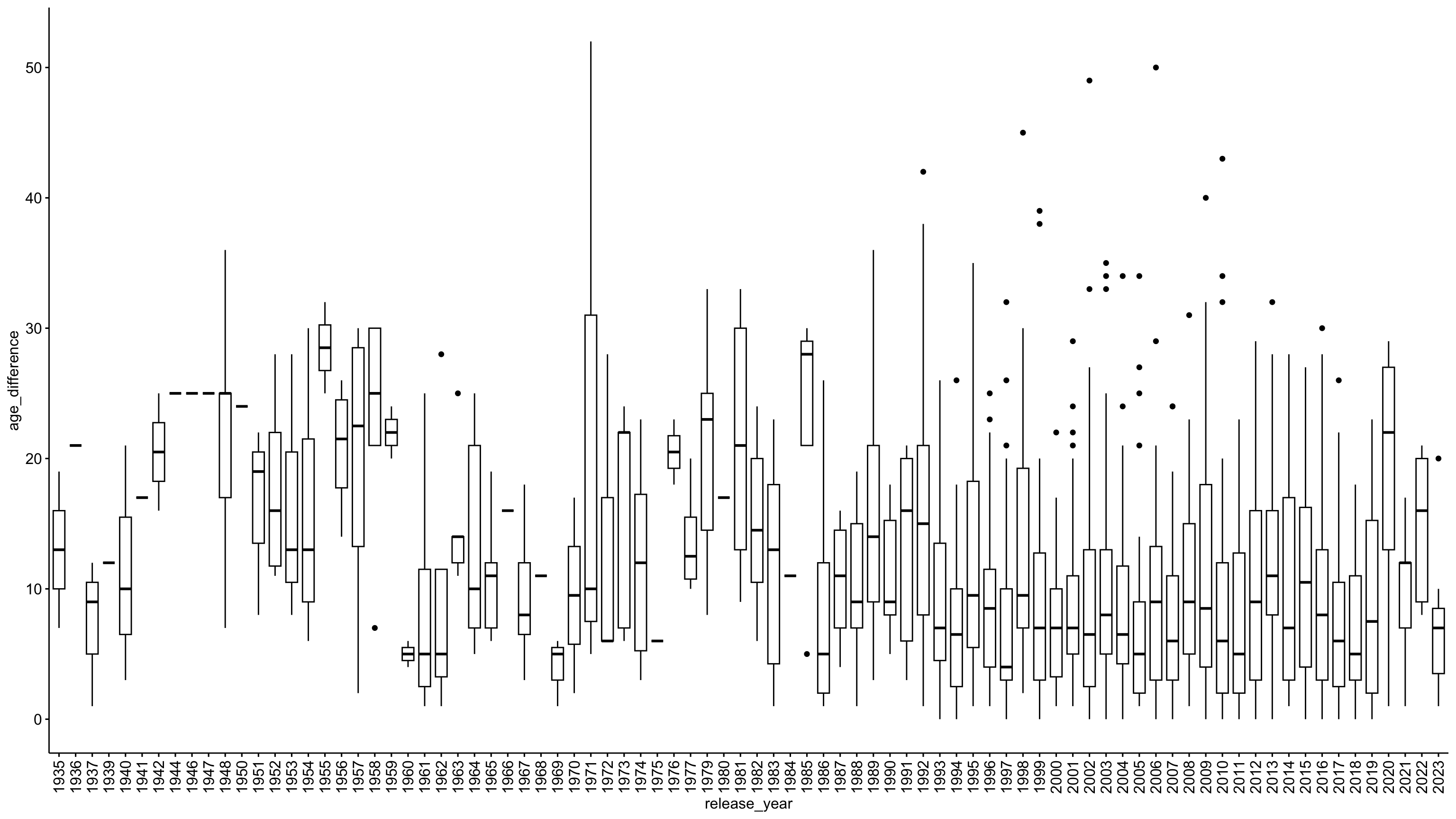
Überprüfung der Korrelation
age_gaps %>%
  select(release_year, age_difference) %>%
  correlation::correlation()
# Correlation Matrix (pearson-method)
Parameter1 | Parameter2 | r | 95% CI | t(1175) | p
----------------------------------------------------------------------------
release_year | age_difference | -0.22 | [-0.27, -0.16] | -7.68 | < .001***
p-value adjustment method: Holm (1979)
Observations: 1177Schätzung OLS
# Schätzung des Models
mdl <- lm(age_difference ~ release_year, data = age_gaps_correct)

# Output
mdl %>% parameters::parameters()
Parameter | Coefficient | SE | 95% CI | t(1175) | p
------------------------------------------------------------------------
(Intercept) | 234.30 | 29.15 | [177.11, 291.50] | 8.04 | < .001
release year | -0.11 | 0.01 | [ -0.14, -0.08] | -7.68 | < .001mdl %>% performance::model_performance()# Indices of model performance
AIC | AICc | BIC | R2 | R2 (adj.) | RMSE | Sigma
------------------------------------------------------------------
8334.623 | 8334.643 | 8349.835 | 0.048 | 0.047 | 8.324 | 8.331mdl %>% report::report()We fitted a linear model (estimated using OLS) to predict age_difference with
release_year (formula: age_difference ~ release_year). The model explains a
statistically significant and weak proportion of variance (R2 = 0.05, F(1,
1175) = 58.96, p < .001, adj. R2 = 0.05). The model's intercept, corresponding
to release_year = 0, is at 234.30 (95% CI [177.11, 291.50], t(1175) = 8.04, p <
.001). Within this model:
- The effect of release year is statistically significant and negative (beta =
-0.11, 95% CI [-0.14, -0.08], t(1175) = -7.68, p < .001; Std. beta = -0.22, 95%
CI [-0.27, -0.16])
Standardized parameters were obtained by fitting the model on a standardized
version of the dataset. 95% Confidence Intervals (CIs) and p-values were
computed using a Wald t-distribution approximation.📋 Exercise: Welche Rolle spielt das Geschlecht?
Spielt das Geschlecht eine Rolle?
- Der folgende Abschitt befasst sich nun ergänzend mit der Frage, welche Rolle das Geschlecht mit Blick auf die “Gültigkeit” der vorherigen Ergebnisse spielt
- Dazu sind jedoch weitere Explorations- und Überarbeitungsschritte notwendig
Übeprüfung der _gender-Variablen
Exercise 1
Nutzen Sie die Funktion sjmisc::frq() und schauen Sie sich im Datensatz age_gaps_correct die Variablen actor_1_gender und actor_2_gender an.
age_gaps_correct %>%
  frq(actor_1_gender, actor_2_gender)
actor_1_gender <character>
# total N=1177 valid N=1177 mean=1.01 sd=0.11
Value | N | Raw % | Valid % | Cum. %
---------------------------------------
man | 1162 | 98.73 | 98.73 | 98.73
woman | 15 | 1.27 | 1.27 | 100.00
<NA> | 0 | 0.00 | <NA> | <NA>
actor_2_gender <character>
# total N=1177 valid N=1177 mean=1.99 sd=0.12
Value | N | Raw % | Valid % | Cum. %
---------------------------------------
man | 16 | 1.36 | 1.36 | 1.36
woman | 1161 | 98.64 | 98.64 | 100.00
<NA> | 0 | 0.00 | <NA> | <NA>
Exercise 2
Nutzen Sie die Funktion sjmisc::flat_talbe() und den Datensatz age_gaps_correct um eine Kreuztabelle der Variablen actor_1_gender und actor_2_gender zu erstellen.
age_gaps_correct %>%
  select(actor_1_gender, actor_2_gender) %>%
  flat_table()
actor_2_gender man woman
actor_1_gender
man 12 1150
woman 4 11Sind die Daten “konsistent”?
Überprüfung der Sortierung
age_gaps_correct %>%
  summarise(
      p1_older = mean(actor_1_age > actor_2_age), # older person first?
      p1_male  = mean(actor_1_gender == "man"),  # male person first?
      p_1_first_alpha = mean(actor_1_name < actor_2_name) # alphabetical order?
  )
# A tibble: 1 × 3
p1_older p1_male p_1_first_alpha
<dbl> <dbl> <dbl>
1 0.811 0.987 0.499Überprüfung der Anzahl pro Paare pro Film
# Create data
couples <- age_gaps_correct %>%
  group_by(movie_name) %>%
  summarise(n = n())

# Distribution
couples %>% frq(n)
n <integer>
# total N=844 valid N=844 mean=1.39 sd=0.75
Value | N | Raw % | Valid % | Cum. %
--------------------------------------
1 | 611 | 72.39 | 72.39 | 72.39
2 | 160 | 18.96 | 18.96 | 91.35
3 | 54 | 6.40 | 6.40 | 97.75
4 | 14 | 1.66 | 1.66 | 99.41
5 | 3 | 0.36 | 0.36 | 99.76
6 | 1 | 0.12 | 0.12 | 99.88
7 | 1 | 0.12 | 0.12 | 100.00
<NA> | 0 | 0.00 | <NA> | <NA># Movies with a loot of couples
couples %>%
filter(n > 3) %>%
arrange(desc(n))# A tibble: 19 × 2
movie_name n
<chr> <int>
1 Love Actually 7
2 The Family Stone 6
3 A View to a Kill 5
4 He's Just Not That Into You 5
5 Mona Lisa Smile 5
6 A Star Is Born 4
7 American Pie 4
8 Boogie Nights 4
9 Book Club 4
10 Closer 4
11 Pushing Tin 4
12 Sex and the City 4
13 Soul Food 4
14 Tag 4
15 The Favourite 4
16 The Girl on the Train 4
17 The Other Woman 4
18 Tomorrow Never Dies 4
19 Twilight 4Korrekturen
age_gaps_consistent <- age_gaps_correct %>%
  # If multiple couples, assign couple number by movie
  mutate(
      couple_number = row_number(),
      .by = "movie_name"
  ) %>%
  # Change data structure (one line per actor in a coulpe of a movie)
  pivot_longer(
    cols = starts_with(c("actor_1_", "actor_2_")),
    names_to = c(NA, NA, ".value"),
    names_sep = "_"
  ) %>%
  # Put older actor first
  arrange(desc(age_difference), movie_name, birthdate) %>%
    mutate(
    position = row_number(),
    .by = c("movie_name", "couple_number")
  ) %>%
  pivot_wider(
    names_from = "position",
    names_glue = "actor_{position}_{.value}",
    values_from = c("name", "gender", "birthdate", "age")
  ) %>%
  mutate(
    couple_structure = case_when(
      actor_1_gender == "woman" & actor_2_gender == "woman" ~ 1,
      actor_1_gender == "man" & actor_2_gender == "man" ~ 2,
      actor_1_gender != "man" ~ 3,
      actor_1_gender == "man" ~ 4,
    ),
    older_male_hetero  = sjmisc::rec(
      couple_structure,
      rec="3=0; 4=1; ELSE=NA",
      to.factor = TRUE
    )
  )
Die zweite Datenexploration
Alterskombinationen im Überblick
Exercise 3
Nutzen Sie die Funktion sjmisc::frq() und schauen Sie sich im Datensatz age_gaps_consistent die Variablen couple_structure und older_male_hetero an.
age_gaps_consistent %>%
  frq(couple_structure, older_male_hetero)
couple_structure <numeric>
# total N=1177 valid N=1177 mean=3.77 sd=0.50
Value | N | Raw % | Valid % | Cum. %
--------------------------------------
1 | 11 | 0.93 | 0.93 | 0.93
2 | 12 | 1.02 | 1.02 | 1.95
3 | 209 | 17.76 | 17.76 | 19.71
4 | 945 | 80.29 | 80.29 | 100.00
<NA> | 0 | 0.00 | <NA> | <NA>
older_male_hetero <categorical>
# total N=1177 valid N=1154 mean=0.82 sd=0.39
Value | N | Raw % | Valid % | Cum. %
--------------------------------------
0 | 209 | 17.76 | 18.11 | 18.11
1 | 945 | 80.29 | 81.89 | 100.00
<NA> | 23 | 1.95 | <NA> | <NA>Wie sind die Altersunterschiede unterteilt, unter Berücksichtiung des Geschlechts?
Graphische Überprüfung
Exercise 4
- Erstellen Sie, auf Basis des Datensatzes
age_gaps_consistent, einenggplot. - Nutzen Sie im Argument
aes()die Variableage_differencealsx-Variable undolder_male_heterofür das Argumentfill. - Nutzen Sie
geom_barzur Erzeugung des Plots. - Optional: Verwenden Sie
theme_pubr
age_gaps_consistent %>%
  ggplot(aes(age_difference, fill = older_male_hetero)) +
  geom_bar() +
  theme_pubr()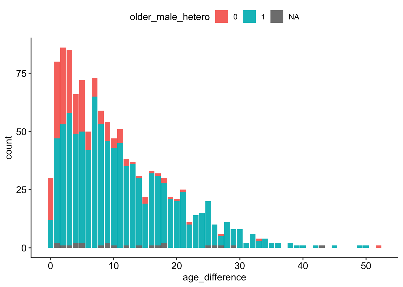
age_gaps_consistent %>%
  ggplot(aes(age_difference, fill = older_male_hetero)) +
  geom_bar() +
  labs(
    x = "Altersdifferenz (in Jahren)",
    y = 'Anzahl der "Beziehungen"'
  ) +
   scale_fill_manual(
    name = "Older partner in couple",
    values = c("0" = "#F8766D", "1" = "#00BFC4", "NA" = "grey"),
    labels = c("0" = "Woman", "1" = "Man", "NA" = "Same sex couples")
  ) +
theme_pubr() 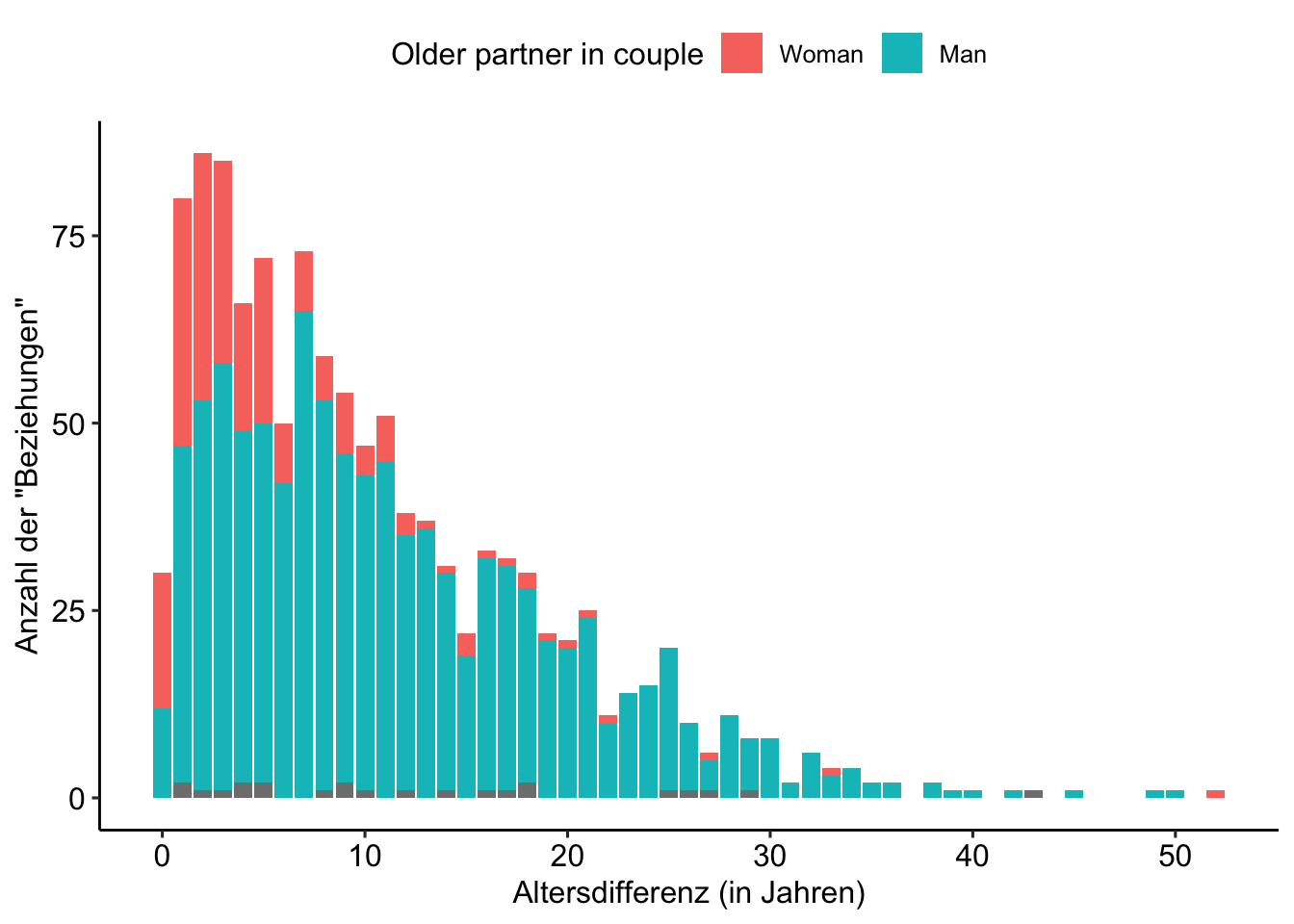
Überprüfung durch Modellierung
mdl <- lm(age_difference ~ release_year + older_male_hetero, data = age_gaps_consistent)

# Output
mdl %>% parameters::parameters()
Parameter | Coefficient | SE | 95% CI | t(1151) | p
---------------------------------------------------------------------------------
(Intercept) | 204.26 | 28.14 | [149.04, 259.47] | 7.26 | < .001
release year | -0.10 | 0.01 | [ -0.13, -0.07] | -7.08 | < .001
older male hetero [1] | 6.03 | 0.61 | [ 4.83, 7.23] | 9.87 | < .001mdl %>% performance::model_performance()# Indices of model performance
AIC | AICc | BIC | R2 | R2 (adj.) | RMSE | Sigma
------------------------------------------------------------------
8058.980 | 8059.015 | 8079.184 | 0.126 | 0.125 | 7.920 | 7.930mdl %>% report::report()We fitted a linear model (estimated using OLS) to predict age_difference with
release_year and older_male_hetero (formula: age_difference ~ release_year +
older_male_hetero). The model explains a statistically significant and weak
proportion of variance (R2 = 0.13, F(2, 1151) = 83.25, p < .001, adj. R2 =
0.12). The model's intercept, corresponding to release_year = 0 and
older_male_hetero = 0, is at 204.26 (95% CI [149.04, 259.47], t(1151) = 7.26, p
< .001). Within this model:
- The effect of release year is statistically significant and negative (beta =
-0.10, 95% CI [-0.13, -0.07], t(1151) = -7.08, p < .001; Std. beta = -0.20, 95%
CI [-0.25, -0.14])
- The effect of older male hetero [1] is statistically significant and positive
(beta = 6.03, 95% CI [4.83, 7.23], t(1151) = 9.87, p < .001; Std. beta = 0.71,
95% CI [0.57, 0.85])
Standardized parameters were obtained by fitting the model on a standardized
version of the dataset. 95% Confidence Intervals (CIs) and p-values were
computed using a Wald t-distribution approximation.