Exercise 09: 🔨 Text as data in R

Digital disconnection on Twitter

Published

16.01.2024

Open session slides

Download source file

Background

Definition

„Digital disconnection is a deliberate (i.e., chosen by the individual) form of non-use of devices, platforms, features, interactions, and/or messages that occurs with higher or lower frequencies, and for shorter or longer periods of time, after the initial adoption of these technologies, and with the aim of restoring or improving one’s perceived overuse, social interactions, psychological well-being, productivity, privacy and/or perceived usefulness“. (Nassen et al. 2023)

Increasing trend towards more conscious use of digital media (devices), including (deliberate) non-use with the aim to restore or improve psychological well-being (among other factors)
But how do “we” talk about digital detox/disconnection: 💊 drug, 👹 demon or 🍩 donut?

Todays’s data basis: Twitter dataset

Collection of all tweets up to the beginning of 2023 that mention or discuss digital detox (and similar terms) on Twitter (not 𝕏)
Initial query is searching for “digital detox”, “#digitaldetox”, “digital_detox”
Access via official Academic-Twitter-API via academictwitteR (Barrie and Ho 2021) at the beginning of last year

Preparation

if (!require("pacman")) install.packages("pacman")
pacman::p_load(
  here, qs, # file management
  magrittr, janitor, # data wrangling
  easystats, sjmisc, # data analysis
  tidytext, textdata, widyr, # text processing
  ggpubr, ggwordcloud, # visualization
  tidyverse # load last to avoid masking issues
  )

Import and process the data

# Import raw data from local
tweets <- qs::qread(here("local_data/tweets-digital_detox.qs"))$raw %>% 
  janitor::clean_names()

# Initial data processing
tweets_correct <- tweets %>% 
  mutate(
    # reformat and create datetime variables
    across(created_at, ~ymd_hms(.)), # convert to dttm format
    year = year(created_at), 
    month = month(created_at), 
    day = day(created_at), 
    hour = hour(created_at),
    minute = minute(created_at),
    # create addtional variables
    retweet_dy = str_detect(text, "^RT"), # identify retweets
    detox_dy = str_detect(text, "#digitaldetox") 
  ) %>% 
  distinct(tweet_id, .keep_all = TRUE)

# Filter relevant tweets
tweets_detox <- tweets_correct %>% 
  filter(
    detox_dy == TRUE, # only tweets with #digitaldetox
    retweet_dy == FALSE, # no retweets
    lang == "en" # only english tweets
    )

Exercises

Objective of this exercise

Brush up basic knowledge of working with R, tidyverse and ggplot2
Get to know the typical steps of tidy text analysis with tidytext, from tokenisation and summarisation to visualisation.

Attention

Before you start working on the exercise, please make sure to render all the chunks of the section Preparation. You can do this by using the “Run all chunks above”-button of the next chunk.
When in doubt, use the showcase (.qmd or .html) to look at the code chunks used to produce the output of the slides.

📋 Exercise 1: Transform to ‘tidy text’

Define custom stopwords
- Edit the vector remove_custom_stopwords by defining additional words to be deleted based on the analysis presented in the session. (Use | as a logical OR operator in regular expressions. It allows you to specify alternatives, e.g. add |https.)
Create new dataset tweets_tidy_cleaned
- Based on the dataset tweets_detox,
  1. use the str_remove_all function to remove the specified patterns of the remove_custom_stopwords vector. Use the mutate() function to edit the text variable.
  2. Tokenize the ‘text’ column using unnest_tokens.
  3. Filter out stop words using filter and stopwords$words
- Save this transformation by creating a new dataset with the name tweets_tidy_cleaned.
Check if transformation was successful (e.g. by using the print() function)

# Define custom stopwords
remove_custom_stopwords <- "&amp;|&lt;|&gt;|http*|t.c|digitaldetox"

# Create new dataset clean_tidy_tweets
tweets_tidy_cleaned <- tweets_detox %>% 
  mutate(text = str_remove_all(text, remove_custom_stopwords)) %>% 
  tidytext::unnest_tokens("text", text) %>% 
  filter(
    !text %in% tidytext::stop_words$word)

# Check
tweets_tidy_cleaned %>% print()

# A tibble: 476,176 × 37
   tweet_id   user_username text       created_at          in_reply_to_user_id
   <chr>      <chr>         <chr>      <dttm>              <chr>              
 1 5777201122 pblackshaw    blackberry 2009-11-16 22:03:12 <NA>               
 2 5777201122 pblackshaw    iphone     2009-11-16 22:03:12 <NA>               
 3 5777201122 pblackshaw    read       2009-11-16 22:03:12 <NA>               
 4 5777201122 pblackshaw    pew        2009-11-16 22:03:12 <NA>               
 5 5777201122 pblackshaw    report     2009-11-16 22:03:12 <NA>               
 6 5777201122 pblackshaw    teens      2009-11-16 22:03:12 <NA>               
 7 5777201122 pblackshaw    distracted 2009-11-16 22:03:12 <NA>               
 8 5777201122 pblackshaw    driving    2009-11-16 22:03:12 <NA>               
 9 5777201122 pblackshaw    bit.ly     2009-11-16 22:03:12 <NA>               
10 5777201122 pblackshaw    4abr5p     2009-11-16 22:03:12 <NA>               
# ℹ 476,166 more rows
# ℹ 32 more variables: author_id <chr>, lang <chr>, possibly_sensitive <lgl>,
#   conversation_id <chr>, user_created_at <chr>, user_protected <lgl>,
#   user_name <chr>, user_verified <lgl>, user_description <chr>,
#   user_location <chr>, user_url <chr>, user_profile_image_url <chr>,
#   user_pinned_tweet_id <chr>, retweet_count <int>, like_count <int>,
#   quote_count <int>, user_tweet_count <int>, user_list_count <int>, …

📋 Exercise 2: Summarize tokens

Create summarized data
- Based on the dataset tweets_tidy_cleaned, summarize the frequency of the individual tokens by using the count()-function on the variable text. Use the argument sort = TRUE to sort the dataset based on descending frequency of the tokens.
- Save this transformation by creating a new dataset with the name tweets_summarized_cleaned.
Check if transformation was successful by using the print() function.
- Use the argument n = 50 to display the top 50 token (only possible if argument sort = TRUE was used when running the count() function)
Check distribution
- Use the datawizard::describe_distribution() function to check different distribution parameters
Optional: Check results with a wordcloud
- Based on the sorted dataset tweets_summarized_cleaned
  1. Select only the 100 most frequent tokens, using the function top_n()
  2. Create a ggplot()-base with label = text and size = n as aes() and
  3. Use ggwordcloud::geom_text_wordclout() to create the wordcloud.
  4. Use scale_size_are() to adopt the scaling of the wordcloud.
  5. Use theme_minimal() for clean visualisation.

# Create summarized data
tweets_summarized_cleaned <- tweets_tidy_cleaned %>% 
  count(text, sort = TRUE) 

# Preview Top 15 token
tweets_summarized_cleaned %>% 
    print(n = 50)

# A tibble: 87,756 × 2
   text                 n
   <chr>            <int>
 1 digital           8521
 2 detox             6623
 3 time              6001
 4 phone             4213
 5 unplug            4021
 6 day               3020
 7 life              2548
 8 social            2449
 9 mindfulness       2408
10 media             2264
11 week              1848
12 unplugging        1674
13 weekend           1651
14 health            1649
15 hnology           1644
16 mentalhealth      1611
17 smartphone        1610
18 screen            1557
19 nature            1421
20 travel            1411
21 wellbeing         1397
22 break             1386
23 addiction         1355
24 listen            1342
25 kids              1339
26 sleep             1315
27 wellness          1301
28 read              1297
29 tips              1247
30 retreat           1242
31 family            1232
32 discuss           1225
33 socialmedia       1208
34 devices           1184
35 screentime        1183
36 icphenomenallyu   1181
37 offline           1072
38 free              1071
39 days              1068
40 world             1068
41 check             1062
42 5                 1013
43 disconnect        1003
44 feel               980
45 enjoy              950
46 switchoff          949
47 people             941
48 digitalwellbeing   937
49 book               932
50 love               922
# ℹ 87,706 more rows

# Check distribution parameters 
tweets_summarized_cleaned %>%
  datawizard::describe_distribution()

Variable | Mean |    SD | IQR |           Range | Skewness | Kurtosis |     n | n_Missing
-----------------------------------------------------------------------------------------
n        | 5.43 | 62.69 |   0 | [1.00, 8521.00] |    67.71 |  6936.19 | 87756 |         0

# Optional: Check results with a wordcloud
tweets_summarized_cleaned %>% 
    top_n(100) %>% 
    ggplot(aes(label = text, size = n)) +
    ggwordcloud::geom_text_wordcloud() +
    scale_size_area(max_size = 15) +
    theme_minimal()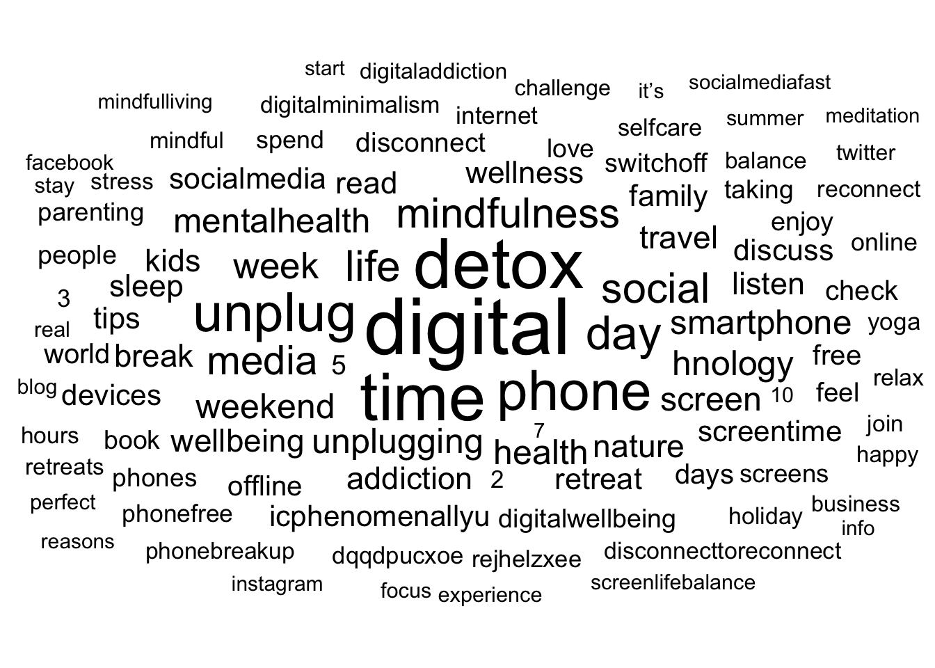

📋 Exercise 3: Couting and correlating pairs of words

3.1 Couting word pairs within tweets

Couting word pairs among sections
- Based on the dataset tweets_tidy_cleaned, count word pairs using widyr::pairwise_count(), with the arguments item = text, feature = tweet_id and sort = TRUE.
- Save this transformation by creating a new dataset with the name tweets_word_pairs_cleand.
Check if transformation was successful by using the print() function.
- Use the argument n = 50 to display the top 50 token (only possible if argument sort = TRUE was used when running the count() function)

# Couting word pairs among sections
tweets_word_pairs_cleand <- tweets_tidy_cleaned %>% 
  widyr::pairwise_count(
    item = text,
    feature = tweet_id,
    sort = TRUE)

# Check 
tweets_word_pairs_cleand %>% print(n = 50)

# A tibble: 2,958,758 × 3
   item1                 item2                     n
   <chr>                 <chr>                 <dbl>
 1 detox                 digital                5195
 2 digital               detox                  5195
 3 media                 social                 1999
 4 social                media                  1999
 5 discuss               listen                 1185
 6 listen                discuss                1185
 7 listen                unplugging             1183
 8 unplugging            listen                 1183
 9 discuss               unplugging             1181
10 icphenomenallyu       unplugging             1181
11 icphenomenallyu       listen                 1181
12 unplugging            discuss                1181
13 icphenomenallyu       discuss                1181
14 unplugging            icphenomenallyu        1181
15 listen                icphenomenallyu        1181
16 discuss               icphenomenallyu        1181
17 time                  digital                 958
18 digital               time                    958
19 screen                time                    883
20 time                  screen                  883
21 unplug                detox                   799
22 detox                 unplug                  799
23 dqqdpucxoe            unplugging              793
24 dqqdpucxoe            listen                  793
25 dqqdpucxoe            discuss                 793
26 dqqdpucxoe            icphenomenallyu         793
27 unplugging            dqqdpucxoe              793
28 listen                dqqdpucxoe              793
29 discuss               dqqdpucxoe              793
30 icphenomenallyu       dqqdpucxoe              793
31 unplug                digital                 791
32 digital               unplug                  791
33 time                  detox                   789
34 detox                 time                    789
35 phonefree             disconnecttoreconnect   682
36 disconnecttoreconnect phonefree               682
37 phonefree             switchoff               673
38 switchoff             phonefree               673
39 digitalminimalism     phonebreakup            636
40 phonebreakup          digitalminimalism       636
41 digitalminimalism     phonefree               633
42 phonefree             digitalminimalism       633
43 time                  unplug                  628
44 unplug                time                    628
45 disconnecttoreconnect switchoff               617
46 switchoff             disconnecttoreconnect   617
47 time                  phone                   616
48 phone                 time                    616
49 phonefree             phonebreakup            615
50 phonebreakup          phonefree               615
# ℹ 2,958,708 more rows

3.2 Pairwise correlation

Getting pairwise correlation
- Based on the dataset tweets_tidy_cleaned,
  1. group the data with the function group_by() by the variable text
  2. use filter(n() >= X) to only use tokens that appear at least a certain amount of times (X).
    Please feel free to select an X of your choice, however, I would strongly recommend an X > 100, as otherwise the following function might not be able to compute.
  3. create word correlations using widyr::pairwise_cor(), with the arguments item = text,feature = tweet_id and sort = TRUE.
- Save this transformation by creating a new dataset with the name tweets_pairs_corr_cleaned.
Check pairs with highest correlation by using the print() function.

# Getting pairwise correlation 
tweets_pairs_corr_cleaned <- tweets_tidy_cleaned %>% 
  group_by(text) %>% 
  filter(n() >= 250) %>% 
  pairwise_cor(text, tweet_id, sort = TRUE)

# Check pairs with highest correlation
tweets_pairs_corr_cleaned %>% print(n = 50)

# A tibble: 62,250 × 3
   item1             item2             correlation
   <chr>             <chr>                   <dbl>
 1 jocelyn           brewer                  0.999
 2 brewer            jocelyn                 0.999
 3 jocelyn           discusses               0.983
 4 discusses         jocelyn                 0.983
 5 igjzl0z4b7        locally                 0.982
 6 locally           igjzl0z4b7              0.982
 7 discusses         brewer                  0.982
 8 brewer            discusses               0.982
 9 icphenomenallyu   discuss                 0.981
10 discuss           icphenomenallyu         0.981
11 taniamulry        wealth                  0.979
12 wealth            taniamulry              0.979
13 locally           cabins                  0.977
14 cabins            locally                 0.977
15 igjzl0z4b7        cabins                  0.970
16 cabins            igjzl0z4b7              0.970
17 jocelyn           nutrition               0.968
18 nutrition         jocelyn                 0.968
19 nutrition         brewer                  0.967
20 brewer            nutrition               0.967
21 discusses         nutrition               0.951
22 nutrition         discusses               0.951
23 icphenomenallyu   listen                  0.937
24 listen            icphenomenallyu         0.937
25 discuss           listen                  0.923
26 listen            discuss                 0.923
27 screenlifebalance mindfulliving           0.920
28 mindfulliving     screenlifebalance       0.920
29 limited           locally                 0.919
30 locally           limited                 0.919
31 screenlifebalance socialmediafast         0.915
32 socialmediafast   screenlifebalance       0.915
33 igjzl0z4b7        limited                 0.913
34 limited           igjzl0z4b7              0.913
35 limited           cabins                  0.908
36 cabins            limited                 0.908
37 taniamulry        info                    0.905
38 info              taniamulry              0.905
39 socialmediafast   digitaladdiction        0.904
40 digitaladdiction  socialmediafast         0.904
41 media             social                  0.901
42 social            media                   0.901
43 socialmediafast   mindfulliving           0.893
44 mindfulliving     socialmediafast         0.893
45 jocelyn           digitalnutrition        0.893
46 digitalnutrition  jocelyn                 0.893
47 brewer            digitalnutrition        0.892
48 digitalnutrition  brewer                  0.892
49 wealth            info                    0.891
50 info              wealth                  0.891
# ℹ 62,200 more rows

3.3. Optinal: Visualization

Customize the parameters in the following code chunk:
- selected_words, for defining the words you want to get the correlates for
- number_of_correlates, to vary the number of correlates shown in the graph.
Set #|eval : true to execute chunk

# Define parameters
selected_words <- c("digital")
number_of_correlates <- 5

# Visualize correlates
tweets_pairs_corr_cleaned %>% 
  filter(item1 %in% selected_words) %>% 
  group_by(item1) %>% 
  slice_max(correlation, n = number_of_correlates) %>% 
  ungroup() %>% 
  mutate(item2 = reorder(item2, correlation)) %>% 
  ggplot(aes(item2, correlation)) +
  geom_bar(stat = "identity") +
  facet_wrap(~ item1, scales = "free") +
  coord_flip() +
  theme_minimal()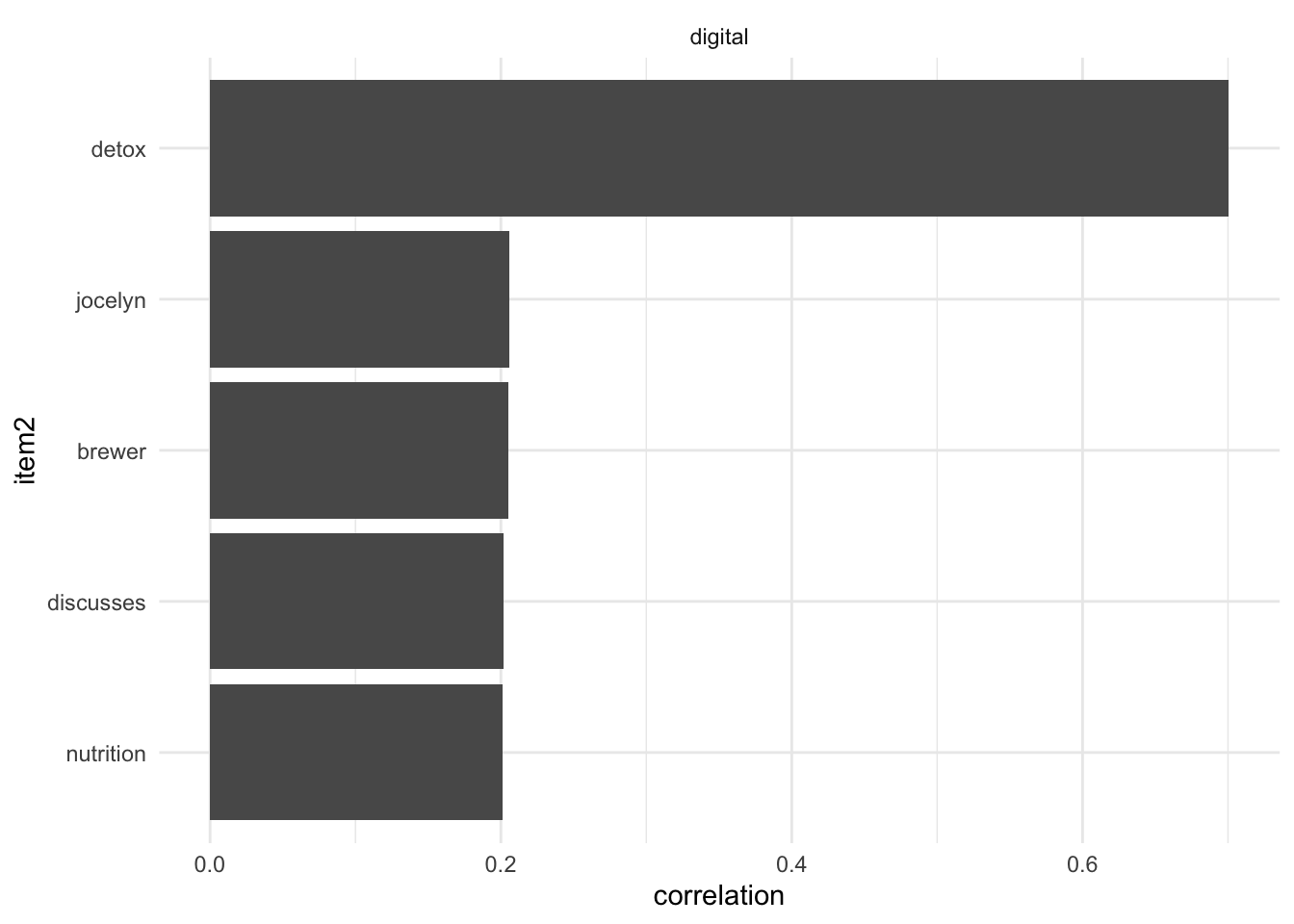

📋 Exercise 4: Sentiment

Apply afinn dictionary to get sentiment
- Based on the dataset tweets_tidy_cleaned,
  1. match the words from the afinn dictionary with the tokens in the tweets by using the inner_join() function. Within inner_join() , please use the get_sentiments() -function with the dictionary "afinn" for y , c("text" = "word") for the by and "many-to-many" for the relationship argument.
  2. use group_by() for grouping the tweets by the variable tweet_id
  3. and summarize() the sentiment for each tweet, by creating a new variable (within the summarize() function), called sentiment, that is the sum (use sum()) of the sentiment values assigned to the words of the dictionary (variable value ).
- Save this transformation by creating a new dataset with the name tweets_sentiment_cleaned.
Check if transformation was successful by using the print() function.
Check distribution
- Use the datawizard::describe_distribution() function to check different distribution parameters
Visualize distribution
- Based on the newly created dataset tweets_sentiment_cleaned, create a ggplot with sentiment as aes() and by using geom_histogram().

# Apply 'afinn' dictionary to get sentiment
tweets_sentiment_cleaned <- tweets_tidy_cleaned %>% 
  inner_join(
     y = get_sentiments("afinn"),
     by = c("text" = "word"),
     relationship = "many-to-many") %>% 
  group_by(tweet_id) %>% 
  summarize(sentiment = sum(value))

# Check transformation
tweets_sentiment_cleaned %>% print()

# A tibble: 23,956 × 2
   tweet_id            sentiment
   <chr>                   <dbl>
 1 1000009901563838465         6
 2 1000038819520008193         1
 3 1000042717492187136        15
 4 1000043574673715203        -1
 5 1000075155891281925         2
 6 1000094334660825088         3
 7 1000104543395315713        -2
 8 1000255467434729472        -1
 9 1000305076286697472         4
10 1000349838595248128         1
# ℹ 23,946 more rows

# Check distribution statistics 
tweets_sentiment_cleaned %>%
  datawizard::describe_distribution()

Variable  | Mean |   SD | IQR |           Range | Skewness | Kurtosis |     n | n_Missing
-----------------------------------------------------------------------------------------
sentiment | 1.24 | 2.77 |   4 | [-13.00, 21.00] |     0.40 |     1.66 | 23956 |         0

# Visualize distribution
tweets_sentiment_cleaned %>% 
  ggplot(aes(sentiment)) +
  geom_histogram() +
  theme_pubr()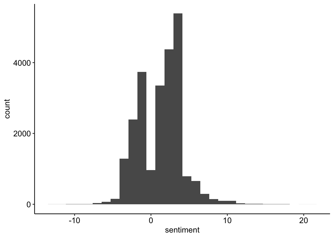

References

Barrie, Christopher, and Justin Ho. 2021. “academictwitteR: An r Package to Access the Twitter Academic Research Product Track V2 API Endpoint.” Journal of Open Source Software 6 (62): 3272. https://doi.org/10.21105/joss.03272.

Nassen, Lise-Marie, Heidi Vandebosch, Karolien Poels, and Kathrin Karsay. 2023. “Opt-Out, Abstain, Unplug. A Systematic Review of the Voluntary Digital Disconnection Literature.” Telematics and Informatics 81 (June): 101980. https://doi.org/10.1016/j.tele.2023.101980.