Showcase 09: 🔨 Text as data in R

Digital disconnection on Twitter

Published

16.01.2024

Open session slides

Background

Definition

„Digital disconnection is a deliberate (i.e., chosen by the individual) form of non-use of devices, platforms, features, interactions, and/or messages that occurs with higher or lower frequencies, and for shorter or longer periods of time, after the initial adoption of these technologies, and with the aim of restoring or improving one’s perceived overuse, social interactions, psychological well-being, productivity, privacy and/or perceived usefulness“. (Nassen et al. 2023)

Increasing trend towards more conscious use of digital media (devices), including (deliberate) non-use with the aim to restore or improve psychological well-being (among other factors)
But how do “we” talk about digital detox/disconnection: 💊 drug, 👹 demon or 🍩 donut?

Todays’s data basis: Twitter dataset

Collection of all tweets up to the beginning of 2023 that mention or discuss digital detox (and similar terms) on Twitter (not 𝕏)
Initial query is searching for “digital detox”, “#digitaldetox”, “digital_detox”
Access via official Academic-Twitter-API via academictwitteR (Barrie and Ho 2021) at the beginning of last year

Preparation

source(here::here("slides/schedule.R"))

if (!require("pacman")) install.packages("pacman")
pacman::p_load(
  here, qs, # file management
  magrittr, janitor, # data wrangling
  easystats, sjmisc, # data analysis
  tidytext, textdata, widyr, # text processing
  ggpubr, ggwordcloud, # visualization
  gt, gtExtras, # fancy tables
  tidyverse # load last to avoid masking issues
  )

Import and process the data

# Import raw data from local
tweets <- qs::qread(here("local_data/tweets-digital_detox.qs"))$raw %>% 
  janitor::clean_names()

# Initial data processing
tweets_correct <- tweets %>% 
  mutate(
    # reformat and create datetime variables
    across(created_at, ~ymd_hms(.)), # convert to dttm format
    year = year(created_at), 
    month = month(created_at), 
    day = day(created_at), 
    hour = hour(created_at),
    minute = minute(created_at),
    # create addtional variables
    retweet_dy = str_detect(text, "^RT"), # identify retweets
    detox_dy = str_detect(text, "#digitaldetox") 
  ) %>% 
  distinct(tweet_id, .keep_all = TRUE)

# Filter relevant tweets
tweets_detox <- tweets_correct %>% 
  filter(
    detox_dy == TRUE, # only tweets with #digitaldetox
    retweet_dy == FALSE, # no retweets
    lang == "en" # only english tweets
    )

Digital disconnection on (not 𝕏)

The structure of the data set & available variables

tweets_correct %>% glimpse()

Rows: 361,408
Columns: 37
$ tweet_id               <chr> "7223508762", "7222271007", "7219735500", "7216…
$ user_username          <chr> "Princessbride24", "winnerandy", "the_enthusias…
$ text                   <chr> "@Ali_Sweeney detox same week as the digital cl…
$ created_at             <dttm> 2009-12-31 05:25:55, 2009-12-31 04:44:20, 2009…
$ in_reply_to_user_id    <chr> "23018333", NA, NA, NA, NA, NA, NA, "19475829",…
$ author_id              <chr> "16157429", "14969949", "16217478", "18001568",…
$ lang                   <chr> "en", "en", "en", "en", "en", "en", "en", "en",…
$ possibly_sensitive     <lgl> FALSE, FALSE, FALSE, FALSE, FALSE, FALSE, FALSE…
$ conversation_id        <chr> "7222577237", "7222271007", "7219735500", "7216…
$ user_created_at        <chr> "2008-09-06T15:13:58.000Z", "2008-06-01T07:34:3…
$ user_protected         <lgl> FALSE, FALSE, FALSE, FALSE, FALSE, FALSE, FALSE…
$ user_name              <chr> "Sam", "Andrew", "The Enthusiast", "🌻BahSun🌻"…
$ user_verified          <lgl> FALSE, FALSE, FALSE, FALSE, FALSE, FALSE, FALSE…
$ user_description       <chr> "As you wish.", "Life is a playground, so enjoy…
$ user_location          <chr> "Houston", "California", "Melbourne, Australia"…
$ user_url               <chr> "https://t.co/hchLJvesW1", NA, "http://t.co/bLK…
$ user_profile_image_url <chr> "https://pbs.twimg.com/profile_images/587051289…
$ user_pinned_tweet_id   <chr> NA, NA, NA, NA, "1285575168010735621", NA, NA, …
$ retweet_count          <int> 0, 0, 0, 0, 0, 0, 0, 0, 0, 0, 0, 0, 0, 0, 0, 0,…
$ like_count             <int> 0, 0, 1, 0, 0, 0, 0, 0, 0, 0, 0, 0, 0, 0, 0, 0,…
$ quote_count            <int> 0, 0, 0, 0, 0, 0, 0, 0, 0, 0, 0, 0, 0, 0, 0, 0,…
$ user_tweet_count       <int> 3905, 18808, 4494, 35337, 284181, 18907, 39562,…
$ user_list_count        <int> 7, 12, 101, 49, 540, 82, 91, 12, 117, 46, 192, …
$ user_followers_count   <int> 103, 481, 2118, 693, 17677, 2527, 8784, 100, 26…
$ user_following_count   <int> 370, 1488, 391, 317, 16470, 320, 11538, 120, 25…
$ sourcetweet_type       <chr> NA, NA, NA, NA, NA, NA, NA, NA, NA, NA, NA, NA,…
$ sourcetweet_id         <chr> NA, NA, NA, NA, NA, NA, NA, NA, NA, NA, NA, NA,…
$ sourcetweet_text       <chr> NA, NA, NA, NA, NA, NA, NA, NA, NA, NA, NA, NA,…
$ sourcetweet_lang       <chr> NA, NA, NA, NA, NA, NA, NA, NA, NA, NA, NA, NA,…
$ sourcetweet_author_id  <chr> NA, NA, NA, NA, NA, NA, NA, NA, NA, NA, NA, NA,…
$ year                   <dbl> 2009, 2009, 2009, 2009, 2009, 2009, 2009, 2009,…
$ month                  <dbl> 12, 12, 12, 12, 12, 12, 12, 12, 12, 12, 12, 12,…
$ day                    <int> 31, 31, 31, 31, 30, 30, 30, 29, 28, 28, 27, 27,…
$ hour                   <int> 5, 4, 3, 1, 22, 2, 0, 20, 21, 1, 19, 8, 8, 3, 9…
$ minute                 <int> 25, 44, 22, 42, 49, 31, 39, 23, 45, 47, 31, 28,…
$ retweet_dy             <lgl> FALSE, FALSE, FALSE, FALSE, TRUE, FALSE, FALSE,…
$ detox_dy               <lgl> FALSE, FALSE, FALSE, FALSE, FALSE, FALSE, FALSE…

Bonus: Distribution statistics

tweets_correct %>% skimr::skim()

Data summary
Name	Piped data
Number of rows	361408
Number of columns	37
_______________________
Column type frequency:
character	19
logical	5
numeric	12
POSIXct	1
________________________
Group variables	None

Variable type: character

skim_variable	n_missing	complete_rate	min	max	empty	n_unique	whitespace
tweet_id	0	1.00	9	19	0	361408	0
user_username	0	1.00	2	15	0	185679	0
text	0	1.00	13	938	0	343311	0
in_reply_to_user_id	321844	0.11	2	19	0	30993	0
author_id	0	1.00	3	19	0	185679	0
lang	0	1.00	2	3	0	60	0
conversation_id	0	1.00	9	19	0	354482	0
user_created_at	0	1.00	24	24	0	185594	0
user_name	0	1.00	0	50	50	178328	0
user_description	0	1.00	0	353	26741	166383	0
user_location	66727	0.82	1	147	0	51237	65
user_url	103146	0.71	12	58	0	115594	0
user_profile_image_url	0	1.00	0	226	44	182266	0
user_pinned_tweet_id	232501	0.36	4	19	0	56397	0
sourcetweet_type	349949	0.03	6	6	0	1	0
sourcetweet_id	349949	0.03	11	19	0	10480	0
sourcetweet_text	349949	0.03	1	755	0	10283	0
sourcetweet_lang	349949	0.03	2	3	0	42	0
sourcetweet_author_id	349949	0.03	2	19	0	7419	0

Variable type: logical

skim_variable	complete_rate	mean	count
possibly_sensitive	1	0.01	FAL: 359068, TRU: 2340
user_protected	1	0.00	FAL: 361408
user_verified	1	0.06	FAL: 340005, TRU: 21403
retweet_dy	1	0.02	FAL: 354735, TRU: 6673
detox_dy	1	0.16	FAL: 303396, TRU: 58012

Variable type: numeric

skim_variable	complete_rate	mean	sd	p0	p25	p50	p75	p100	hist
retweet_count	1	0.77	21.53	0	0	0	0.00	9035	▇▁▁▁▁
like_count	1	3.17	219.89	0	0	0	1.00	98181	▇▁▁▁▁
quote_count	1	0.09	11.07	0	0	0	0.00	5213	▇▁▁▁▁
user_tweet_count	1	60860.29	173889.51	1	2933	12371	41843.00	9641956	▇▁▁▁▁
user_list_count	1	375.59	2643.28	0	7	46	171.00	216734	▇▁▁▁▁
user_followers_count	1	37077.25	532883.29	0	274	1157	4724.25	61075617	▇▁▁▁▁
user_following_count	1	2952.88	18952.23	0	221	808	2067.00	1407439	▇▁▁▁▁
year	1	2016.96	2.73	2007	2015	2017	2019.00	2022	▁▂▇▇▅
month	1	6.36	3.49	1	3	7	9.00	12	▇▅▅▆▇
day	1	15.50	8.95	1	7	15	23.00	31	▇▆▆▆▆
hour	1	12.62	6.08	0	8	13	17.00	23	▃▅▆▇▅
minute	1	27.09	17.93	0	11	27	43.00	59	▇▆▆▆▆

Variable type: POSIXct

skim_variable	n_missing	complete_rate	min	max	median	n_unique
created_at	0	1	2007-11-19 09:14:10	2022-12-31 23:18:38	2017-04-26 08:15:03	352271

Distribution of tweets with reference to digital detox over time

tweets_correct %>% 
  ggplot(aes(x = as.factor(year), fill = retweet_dy)) +
    geom_bar() +
    labs(
      x = "",
      y = "Number of tweets", 
      fill = "Is the tweet a retweet?"
     ) +
    scale_fill_manual(values = c("#1DA1F2", "#004389")) +
    theme_pubr() +    
    # add annotations
    annotate(
      "text", 
      x = 14, y = 55000,
      label = "Increase of character limit from 140 to 280") + 
    geom_curve(
      data = data.frame(
        x = 14.2965001234837,y = 53507.2283841571,
        xend = 11.5275706534335, yend = 45412.4966032138),
      mapping = aes(x = x, y = y, xend = xend, yend = yend),
      angle = 127L,
      curvature = 0.28,
      arrow = arrow(30L, unit(0.1, "inches"), "last", "closed"),
      inherit.aes = FALSE)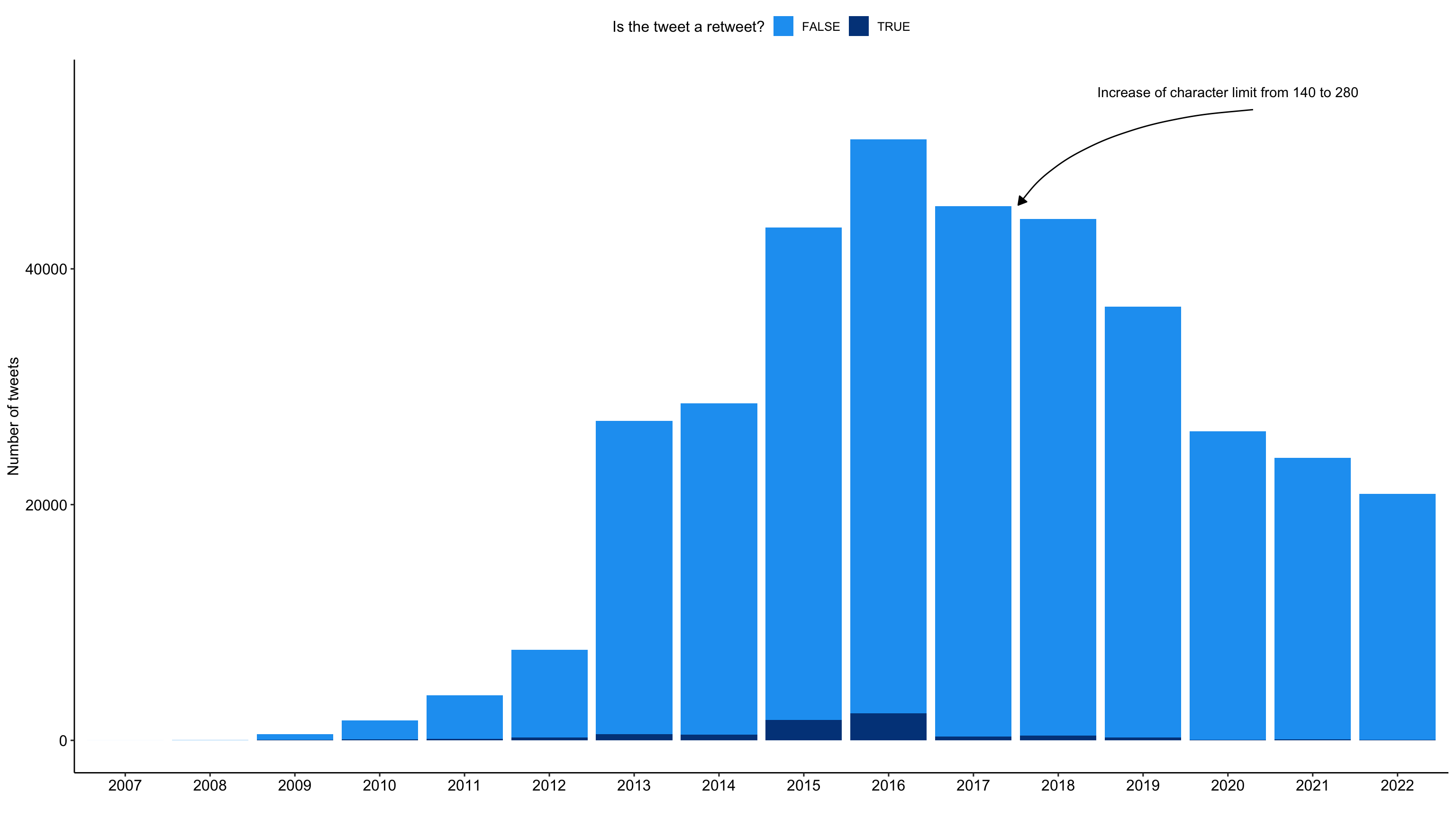

Tweets with reference to ditigal detox by (participating) users

tweets_correct %>% 
    group_by(author_id) %>% 
    summarize(n = n()) %>% 
    mutate(
        n_grp = case_when(
                     n <=    1 ~ 1,
            n >   1 & n <=  10 ~ 2,
            n >  10 & n <=  25 ~ 3,
            n >  25 & n <=  50 ~ 4,
            n >  50 & n <=  75 ~ 5,
            n >  75 & n <= 100 ~ 6,
            n > 100 ~ 7
        ), 
        n_grp_fct = factor(
            n_grp,
            levels = c(1:7),
            labels = c(
            " 1",
            " 2 - 10", "11 - 25",
            "26 - 50", "50 - 75",
            "75 -100", "> 100")
        )
    ) %>% 
    sjmisc::frq(n_grp_fct) %>% 
    as.data.frame() %>% 
    select(val, frq:cum.prc) %>% 
    # create table
    gt() %>% 
    # tab_header(
    #     title = "Tweets by users with a least on tweet"
    #    ) %>% 
    cols_label(
      val = "Number of tweets by user",
      frq = "n",
      raw.prc = html("%<sub>raw</sub>"),
      cum.prc = html("%<sub>cum</sub>")
  ) %>% 
  gt_theme_538()

Number of tweets by user	n	%_raw	%_cum
1	143364	77.21	77.21
2 - 10	39981	21.53	98.74
11 - 25	1647	0.89	99.63
26 - 50	435	0.23	99.86
50 - 75	88	0.05	99.91
75 -100	55	0.03	99.94
> 100	109	0.06	100.00
NA	0	0.00	NA

Tweets with reference to ditigal detox by language

tweets_correct %>% 
    sjmisc::frq(
        lang, 
        sort.frq = c("desc"), 
        min.frq = 2000
    ) %>% 
    as.data.frame() %>% 
    select(val, frq:cum.prc) %>% 
    # create table
    gt() %>% 
    # tab_header(
    #     title = "Language of the collected tweets"
    #   ) %>% 
    cols_label(
      val = "Twitter language code",
      frq = "n",
      raw.prc = html("%<sub>raw</sub>"),
      cum.prc = html("%<sub>cum</sub>")
  ) %>% 
  gt_theme_538()

Twitter language code	n	%_raw	%_cum
en	274351	75.91	75.91
fr	20407	5.65	81.56
es	16248	4.50	86.05
de	14091	3.90	89.95
pt	7127	1.97	91.92
it	5999	1.66	93.58
da	3490	0.97	94.55
in	3095	0.86	95.41
ja	2428	0.67	96.08
n < 2000	14172	3.92	100.00
NA	0	0.00	NA

Text as data in R (Part I)

Build a subsample: Tweets containing #digitaldetox

tweets_detox <- tweets_correct %>% 
  filter(
    detox_dy == TRUE, # only tweets with #digitaldetox
    retweet_dy == FALSE, # no retweets
    lang == "en" # only english tweets
    )

Expand for full code

tweets_correct %>% 
  ggplot(aes(x = as.factor(year), fill = detox_dy)) +
    geom_bar() +
    labs(
      x = "",
      y = "Number of tweets", 
      fill = "#digitaldetox used in tweet?"
     ) +
    scale_fill_manual(values = c("#A0ACBD50", "#1DA1F2")) +
    theme_pubr()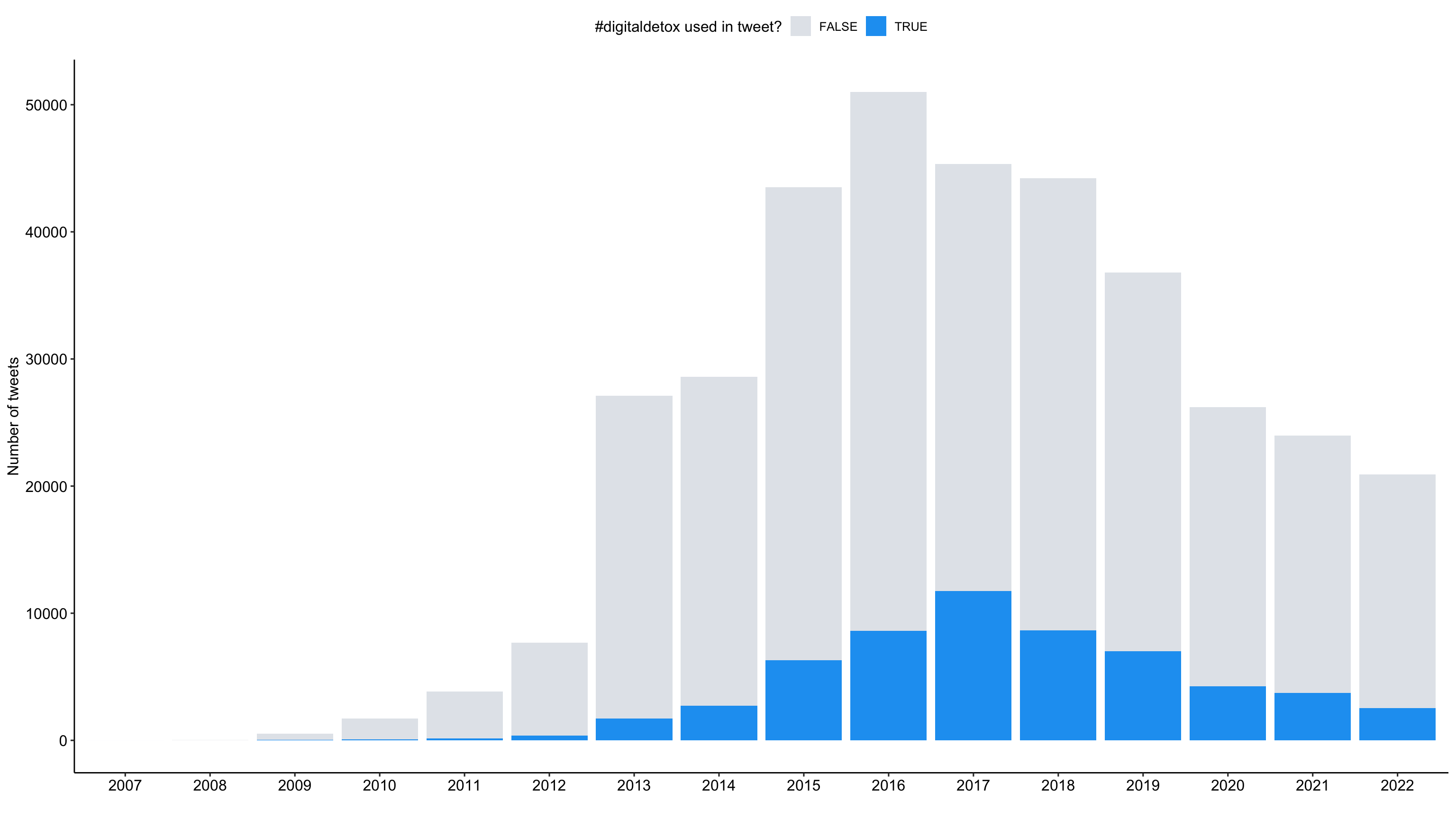

Bonus: distribution statistics

tweets_detox %>% skimr::skim()

Data summary
Name	Piped data
Number of rows	46670
Number of columns	37
_______________________
Column type frequency:
character	19
logical	5
numeric	12
POSIXct	1
________________________
Group variables	None

Variable type: character

skim_variable	n_missing	complete_rate	min	max	empty	n_unique	whitespace
tweet_id	0	1.00	10	19	0	46670	0
user_username	0	1.00	3	15	0	15383	0
text	0	1.00	18	873	0	45039	0
in_reply_to_user_id	43310	0.07	3	19	0	2617	0
author_id	0	1.00	3	19	0	15383	0
lang	0	1.00	2	2	0	1	0
conversation_id	0	1.00	10	19	0	46235	0
user_created_at	0	1.00	24	24	0	15383	0
user_name	0	1.00	1	50	0	15252	0
user_description	0	1.00	0	227	1089	14612	0
user_location	5596	0.88	1	113	0	5834	2
user_url	5863	0.87	18	44	0	11413	0
user_profile_image_url	0	1.00	59	151	0	15317	0
user_pinned_tweet_id	21644	0.54	9	19	0	4756	0
sourcetweet_type	44990	0.04	6	6	0	1	0
sourcetweet_id	44990	0.04	18	19	0	1620	0
sourcetweet_text	44990	0.04	23	402	0	1620	0
sourcetweet_lang	44990	0.04	2	3	0	14	0
sourcetweet_author_id	44990	0.04	4	19	0	1227	0

Variable type: logical

skim_variable	complete_rate	mean	count
possibly_sensitive	1	0.00	FAL: 46559, TRU: 111
user_protected	1	0.00	FAL: 46670
user_verified	1	0.03	FAL: 45200, TRU: 1470
retweet_dy	1	0.00	FAL: 46670
detox_dy	1	1.00	TRU: 46670

Variable type: numeric

skim_variable	complete_rate	mean	sd	p0	p25	p50	p75	p100	hist
retweet_count	1	0.70	30.82	0	0.00	0.0	0	6618	▇▁▁▁▁
like_count	1	2.88	220.54	0	0.00	0.0	1	47308	▇▁▁▁▁
quote_count	1	0.06	1.62	0	0.00	0.0	0	340	▇▁▁▁▁
user_tweet_count	1	27905.41	76117.39	1	1809.00	10199.0	16045	1268964	▇▁▁▁▁
user_list_count	1	208.86	557.75	0	15.00	109.0	163	25072	▇▁▁▁▁
user_followers_count	1	7627.12	74560.68	0	519.25	2410.0	5032	7977533	▇▁▁▁▁
user_following_count	1	2223.94	6345.92	0	398.00	1749.5	1989	475935	▇▁▁▁▁
year	1	2017.40	2.24	2009	2016.00	2017.0	2019	2022	▁▂▅▇▃
month	1	6.43	3.48	1	3.00	7.0	9	12	▇▅▅▆▇
day	1	15.58	8.77	1	8.00	16.0	23	31	▇▆▇▆▆
hour	1	12.50	5.52	0	9.00	13.0	16	23	▂▅▆▇▃
minute	1	24.62	17.97	0	7.00	25.0	39	59	▇▅▆▃▃

Variable type: POSIXct

skim_variable	n_missing	complete_rate	min	max	median	n_unique
created_at	0	1	2009-01-04 12:10:04	2022-12-31 21:23:34	2017-09-08 10:45:05	46448

Transform data to tidy text

# Common HTML entities
remove_reg <- "&amp;|&lt;|&gt;"

# Create tidy data
tweets_tidy <- tweets_detox %>% 
    # Remove HTML entities
    mutate(text = str_remove_all(text, remove_reg)) %>% 
    # Tokenization
    tidytext::unnest_tokens("text", text) %>% 
    # Remove stopwords
    filter(!text %in% tidytext::stop_words$word)

# Preview
tweets_tidy %>% 
    select(tweet_id, user_username, text) %>% 
    print(n = 5)

# A tibble: 639,459 × 3
  tweet_id   user_username text      
  <chr>      <chr>         <chr>     
1 5777201122 pblackshaw    blackberry
2 5777201122 pblackshaw    iphone    
3 5777201122 pblackshaw    read      
4 5777201122 pblackshaw    pew       
5 5777201122 pblackshaw    report    
# ℹ 639,454 more rows

Summarize all tokens over all tweets

# Create summarized data
tweets_summarized <- tweets_tidy %>% 
  count(text, sort = TRUE) 

# Preview Top 15 token
tweets_summarized %>% 
    print(n = 15)

# A tibble: 87,172 × 2
   text             n
   <chr>        <int>
 1 t.co         57530
 2 https        52890
 3 digitaldetox 46642
 4 digital       8521
 5 detox         6623
 6 time          6000
 7 http          4674
 8 phone         4213
 9 unplug        4021
10 day           2939
11 life          2548
12 social        2449
13 mindfulness   2408
14 media         2264
15 technology    2065
# ℹ 87,157 more rows

Visualization of Top 100 token

tweets_summarized %>% 
    top_n(100) %>% 
    ggplot(aes(label = text, size = n)) +
    ggwordcloud::geom_text_wordcloud() +
    scale_size_area(max_size = 30) +
    theme_minimal()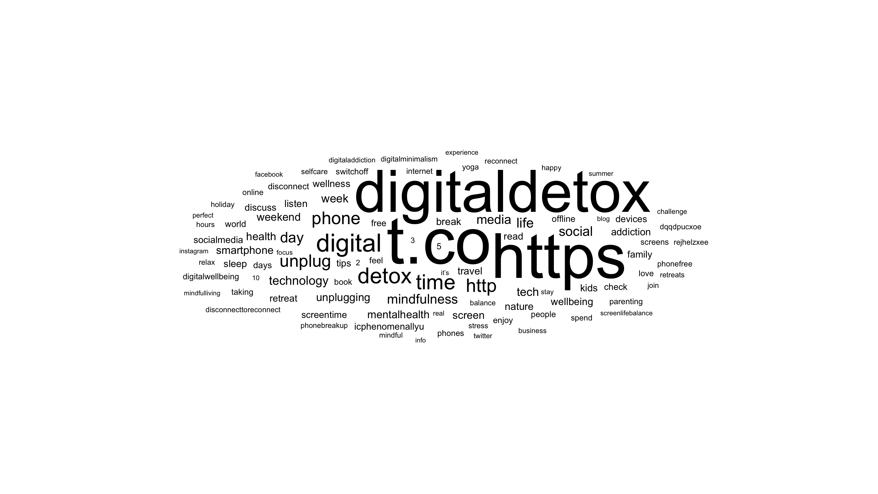

Modeling realtionships between words

Count word pairs within tweets

# Create word paris
tweets_word_pairs <- tweets_tidy %>% 
    widyr::pairwise_count(
        text,
        tweet_id,
        sort = TRUE)

# Preview
tweets_word_pairs %>% 
    print(n = 15)

# A tibble: 3,466,216 × 3
   item1        item2            n
   <chr>        <chr>        <dbl>
 1 t.co         digitaldetox 40640
 2 digitaldetox t.co         40640
 3 t.co         https        36605
 4 https        t.co         36605
 5 https        digitaldetox 36486
 6 digitaldetox https        36486
 7 digital      digitaldetox  7791
 8 digitaldetox digital       7791
 9 t.co         digital       7365
10 digital      t.co          7365
11 https        digital       6856
12 digital      https         6856
13 detox        digitaldetox  6004
14 digitaldetox detox         6004
15 t.co         detox         5672
# ℹ 3,466,201 more rows

Summarize and correlate tokens within tweets

# Create word correlation
tweets_pairs_corr <- tweets_tidy %>% 
    group_by(text) %>% 
    filter(n() >= 300) %>% 
    pairwise_cor(
        text, 
        tweet_id, 
        sort = TRUE)

# Preview
tweets_pairs_corr %>% 
    print(n = 15)

# A tibble: 41,820 × 3
   item1           item2           correlation
   <chr>           <chr>                 <dbl>
 1 jocelyn         brewer                0.999
 2 brewer          jocelyn               0.999
 3 jocelyn         discusses             0.983
 4 discusses       jocelyn               0.983
 5 discusses       brewer                0.982
 6 brewer          discusses             0.982
 7 icphenomenallyu discuss               0.981
 8 discuss         icphenomenallyu       0.981
 9 taniamulry      wealth                0.979
10 wealth          taniamulry            0.979
11 jocelyn         nutrition             0.968
12 nutrition       jocelyn               0.968
13 nutrition       brewer                0.967
14 brewer          nutrition             0.967
15 discusses       nutrition             0.951
# ℹ 41,805 more rows

Display correlates for specific token

tweets_pairs_corr %>% 
  filter(
    item1 %in% c("detox", "digital")
    ) %>% 
  group_by(item1) %>% 
  slice_max(correlation, n = 5) %>% 
  ungroup() %>% 
  mutate(
    item2 = reorder(item2, correlation)
    ) %>% 
  ggplot(
    aes(item2, correlation, fill = item1)
    ) +
  geom_bar(stat = "identity") +
  facet_wrap(~ item1, scales = "free") +
  coord_flip() +
  scale_fill_manual(
    values = c("#C50F3C", "#04316A")) +
  theme_pubr()

Dictionary based approach: Sentiment analysis

Most commmon positive and negative words

tweets_sentiment_count <- tweets_tidy %>% 
  inner_join(
     get_sentiments("bing"),
     by = c("text" = "word"),
     relationship = "many-to-many") %>% 
  count(text, sentiment)
  
# Preview
tweets_sentiment_count %>% 
  group_by(sentiment) %>%
  slice_max(n, n = 10) %>% 
  ungroup() %>% 
  mutate(text = reorder(text, n)) %>%
  ggplot(aes(n, text, fill = sentiment)) +
  geom_col(show.legend = FALSE) +
  facet_wrap(
    ~sentiment, scales = "free_y") +
  labs(x = "Contribution to sentiment",
       y = NULL) +
  scale_fill_manual(
    values = c("#C50F3C", "#007D29")) +
  theme_pubr()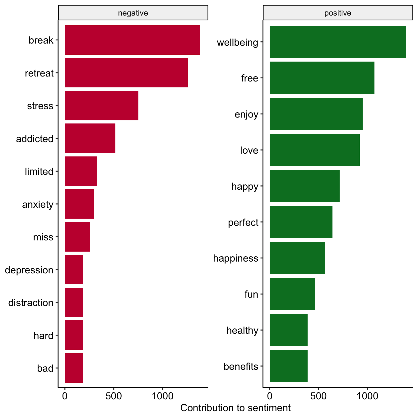

Link word sentiment to tidy data

tweets_sentiment <- tweets_tidy %>% 
  inner_join(
     get_sentiments("bing"),
     by = c("text" = "word"),
     relationship = "many-to-many") %>% 
  count(tweet_id, sentiment) %>% 
  pivot_wider(names_from = sentiment, values_from = n, values_fill = 0) %>% 
  mutate(sentiment = positive - negative)
  
# Check
tweets_sentiment

# A tibble: 24,372 × 4
   tweet_id            positive negative sentiment
   <chr>                  <int>    <int>     <int>
 1 1000009901563838465        3        0         3
 2 1000038819520008193        1        0         1
 3 1000042717492187136        4        0         4
 4 1000043574673715203        1        1         0
 5 1000075155891281925        4        0         4
 6 1000086637987139590        1        0         1
 7 1000094334660825088        1        0         1
 8 1000133715194920960        1        0         1
 9 1000255467434729472        0        1        -1
10 1000271209353895938        1        1         0
# ℹ 24,362 more rows

Overall distribution sentiment by tweets

tweets_sentiment %>% 
  ggplot(aes(as.factor(sentiment))) +
  geom_bar(fill = "#1DA1F2") +
  labs(
    x = "Sentiment (sum) of tweet", 
    y = "Number of tweets"
  ) +
  theme_pubr()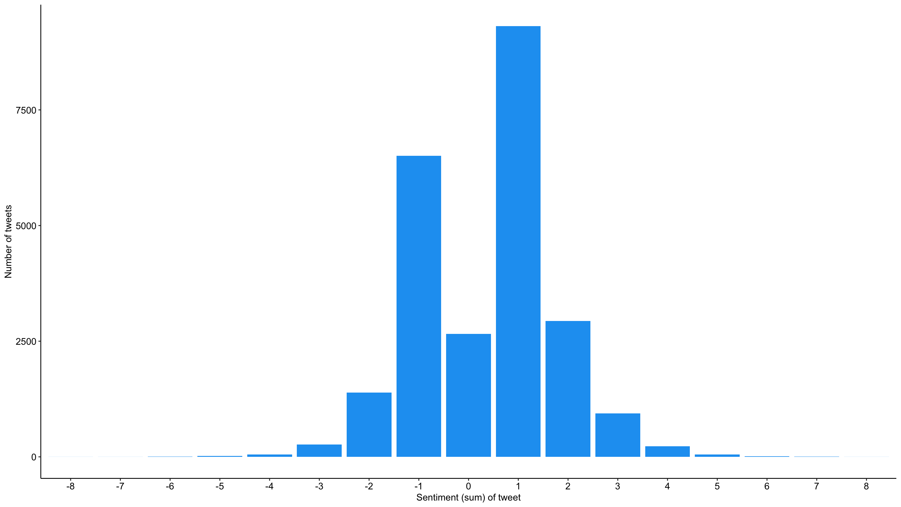

Development of tweet sentiment over the years

Expand for full code

# Create first graph
g1 <- tweets_correct %>% 
  filter(tweet_id %in% tweets_sentiment$tweet_id) %>% 
  left_join(tweets_sentiment) %>% 
  sjmisc::rec(
    sentiment,
    rec = "-8:-1=negative; 0=neutral; 1:8=positive") %>%
  ggplot(aes(x = as.factor(year), fill = as.factor(sentiment_r))) +
    geom_bar() +
    labs(
      x = "",
      y = "Number of tweets", 
      fill = "Sentiment (sum) of tweet") +
    scale_fill_manual(values = c("#C50F3C", "#90A0AF", "#007D29")) +
    theme_pubr() 
    #theme(axis.text.x = element_text(angle = 90, vjust = 0.5, hjust=1))

# Create second graph
g2 <- tweets_correct %>% 
  filter(tweet_id %in% tweets_sentiment$tweet_id) %>% 
  left_join(tweets_sentiment) %>% 
  sjmisc::rec(
    sentiment,
    rec = "-8:-1=negative; 0=neutral; 1:8=positive") %>%
  ggplot(aes(x = as.factor(year), fill = as.factor(sentiment_r))) +
    geom_bar(position = "fill") +
    labs(
      x = "",
      y = "Proportion of tweets", 
      fill = "Sentiment (sum) of tweet") +
    scale_fill_manual(values = c("#C50F3C", "#90A0AF", "#007D29")) +
    theme_pubr() 

# COMBINE GRPAHS
ggarrange(g1, g2,
          nrow = 1, ncol = 2, 
          align = "hv",
          common.legend = TRUE)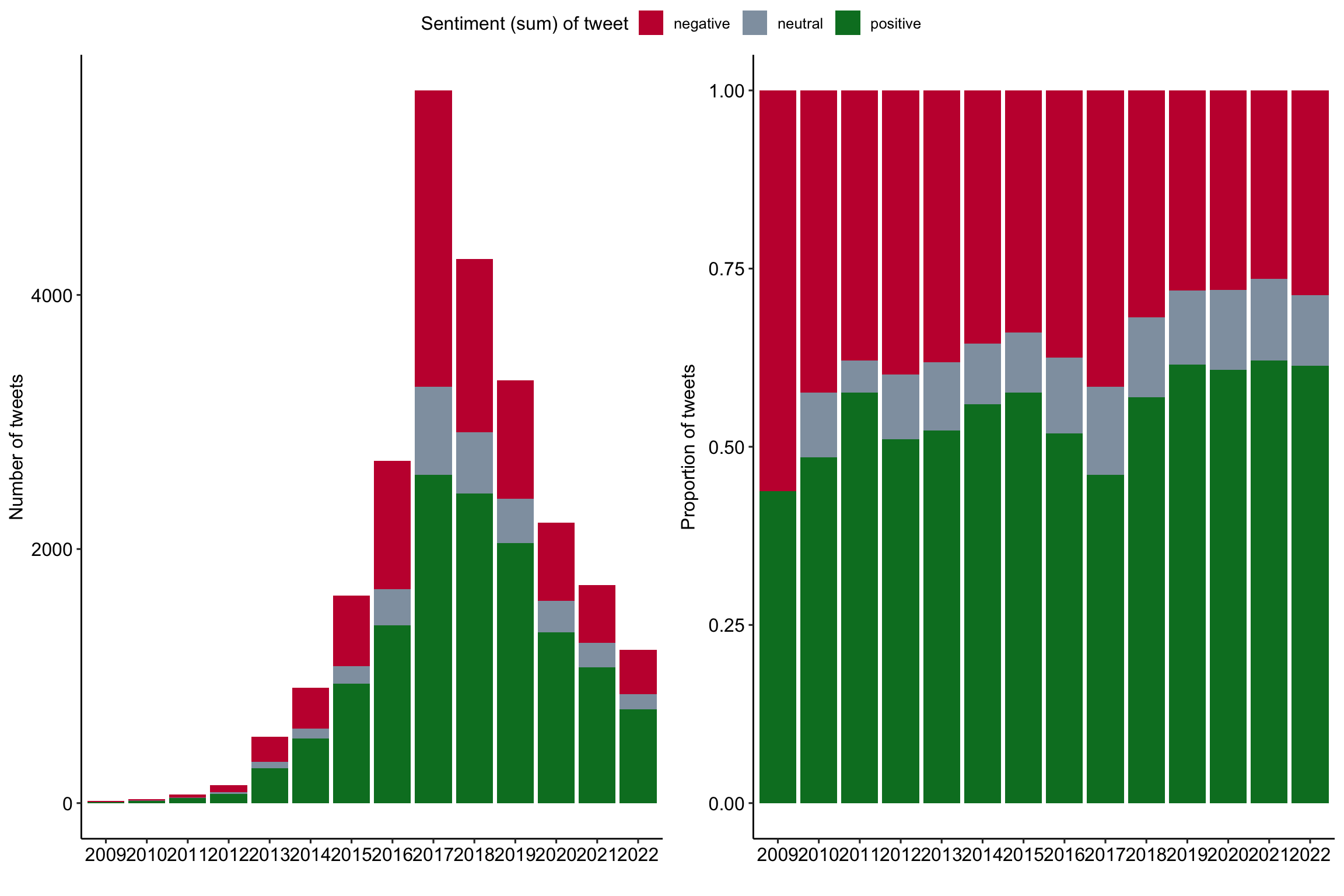

References

Barrie, Christopher, and Justin Ho. 2021. “academictwitteR: An r Package to Access the Twitter Academic Research Product Track V2 API Endpoint.” Journal of Open Source Software 6 (62): 3272. https://doi.org/10.21105/joss.03272.

Nassen, Lise-Marie, Heidi Vandebosch, Karolien Poels, and Kathrin Karsay. 2023. “Opt-Out, Abstain, Unplug. A Systematic Review of the Voluntary Digital Disconnection Literature.” Telematics and Informatics 81 (June): 101980. https://doi.org/10.1016/j.tele.2023.101980.