if (!require("pacman")) install.packages("pacman")
pacman::p_load(
  here, qs, # file management
  magrittr, janitor, # data wrangling
  easystats, sjmisc, # data analysis
  ggpubr, ggwordcloud, # visualization
  gt, gtExtras, # fancy tables
  tidytext, textdata, widyr, # tidy text processing
  quanteda, # quanteda text processing
  quanteda.textplots,
  topicmodels, stm,
  tidyverse # load last to avoid masking issues
)Showcase 10: 🔨 Automatic analysis of text in R
Digital disconnection on Twitter
![]() Open session slides
Open session slides
Background
Increasing trend towards more conscious use of digital media (devices), including (deliberate) non-use with the aim to restore or improve psychological well-being (among other factors)
But how do “we” talk about digital detox/disconnection: 💊 drug, 👹 demon or 🍩 donut?
Todays’s data basis: Twitter dataset
- Collection of all tweets up to the beginning of 2023 that mention or discuss digital detox (and similar terms) on Twitter (not 𝕏)
- Initial query is searching for “digital detox”, “#digitaldetox”, “digital_detox”
- Access via official Academic-Twitter-API via academictwitteR (Barrie and Ho 2021) at the beginning of last year
Preparation
Import and process the data
# Import raw data from local
tweets <- qs::qread(here("local_data/tweets-digital_detox.qs"))$raw %>%
  janitor::clean_names()

# Initial data processing
tweets_correct <- tweets %>%
  mutate(
    # reformat and create datetime variables
    across(created_at, ~ymd_hms(.)), # convert to dttm format
    year = year(created_at),
    month = month(created_at),
    day = day(created_at),
    hour = hour(created_at),
    minute = minute(created_at),
    # create addtional variables
    retweet_dy = str_detect(text, "^RT"), # identify retweets
    detox_dy = str_detect(text, "#digitaldetox")
  ) %>%
  distinct(tweet_id, .keep_all = TRUE)

# Filter relevant tweets
tweets_detox <- tweets_correct %>%
  filter(
    detox_dy == TRUE, # only tweets with #digitaldetox
    retweet_dy == FALSE, # no retweets
    lang == "en" # only english tweets
    )

# Topic models
stm_k0 <- qs::qread(here("local_data/stm_k0.qs"))
stm_exploration <- qs::qread(here("local_data/stm_exploration.qs"))
stm_results <- qs::qread(here("local_data/stm_results.qs"))
Text as data in R (Part II)
Step-by-step DTM creation
# Common HTML entities
remove_reg <- "&|<|>"
# Create tidy data
tweets_tidy <- tweets_detox %>%
mutate(
text = str_remove_all(text, remove_reg)) %>%
tidytext::unnest_tokens("text", text) %>%
filter(!text %in% tidytext::stop_words$word)
# Create summarized data
tweets_summarized <- tweets_tidy %>%
count(tweet_id, text)
# Create DTM
tweets_dfm <- tweets_summarized %>%
cast_dfm(tweet_id, text, n)
# Preview
tweets_dfmDocument-feature matrix of: 46,670 documents, 87,172 features (99.99% sparse) and 0 docvars.
features
docs bite detox digital digitaldetox enjoy fly happitizer
1000009901563838465 1 1 1 1 2 1 1
1000038819520008193 0 0 0 1 0 0 0
1000042717492187136 0 0 0 1 0 0 0
1000043574673715203 0 0 0 1 0 0 0
1000053895035531264 0 1 1 1 0 0 0
1000075155891281925 0 0 0 1 0 0 0
features
docs happitizers https inspiration
1000009901563838465 1 1 1
1000038819520008193 0 1 0
1000042717492187136 0 1 0
1000043574673715203 0 2 0
1000053895035531264 0 2 0
1000075155891281925 0 1 0
[ reached max_ndoc ... 46,664 more documents, reached max_nfeat ... 87,162 more features ]# Create corpus
quanteda_corpus <- tweets_detox %>%
quanteda::corpus(
docid_field = "tweet_id",
text_field = "text"
)
# Tokenize
quanteda_token <- quanteda_corpus %>%
quanteda::tokens(
remove_punct = TRUE,
remove_symbols = TRUE,
remove_numbers = TRUE,
remove_url = TRUE,
split_tags = FALSE # keep hashtags and mentions
) %>%
quanteda::tokens_tolower() %>%
quanteda::tokens_remove(
pattern = stopwords("en")
)
# Convert to Document-Feature-Matrix (DFM)
quanteda_dfm <- quanteda_token %>%
quanteda::dfm()
# Preview
quanteda_dfmDocument-feature matrix of: 46,670 documents, 49,123 features (99.98% sparse) and 35 docvars.
features
docs put blackberry iphone read pew report teens distracted driving
5777201122 1 1 1 1 1 1 1 1 1
4814687834 0 0 0 0 0 0 0 0 0
4813781509 0 0 0 0 0 0 0 0 0
3351604894 0 0 0 0 0 0 0 0 0
3350930292 0 0 0 0 0 0 0 0 0
3349372574 0 0 0 0 0 0 0 0 0
features
docs #digitaldetox
5777201122 1
4814687834 1
4813781509 1
3351604894 1
3350930292 1
3349372574 1
[ reached max_ndoc ... 46,664 more documents, reached max_nfeat ... 49,113 more features ]Network of hashtags
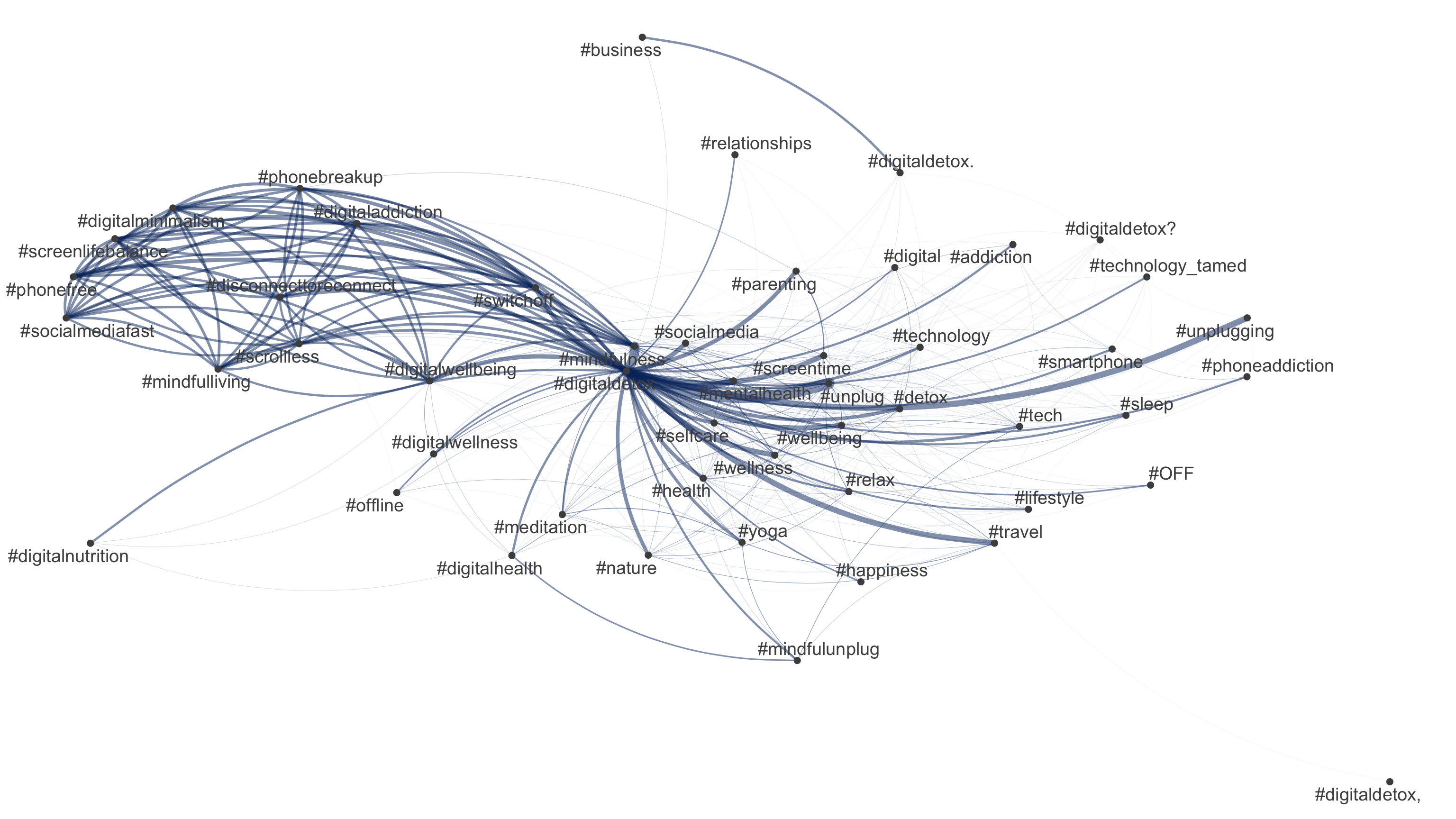
# Extract hashtags
tweets_hashtags <- tweets_detox %>%
  mutate(hashtags = str_extract_all(text, "#\\S+")) %>%
  unnest(hashtags)

# Extract most common hashtags
top50_hashtags_tidy <- tweets_hashtags %>%
  count(hashtags, sort = TRUE) %>%
  slice_head(n = 50) %>%
  pull(hashtags)

# Visualize
tweets_hashtags %>%
  count(tweet_id, hashtags, sort = TRUE) %>%
  cast_dfm(tweet_id, hashtags, n) %>%
  quanteda::fcm() %>%
  quanteda::fcm_select(
    pattern = top50_hashtags_tidy,
    case_insensitive = FALSE
    ) %>%
  quanteda.textplots::textplot_network(
    edge_color = "#04316A"
  )
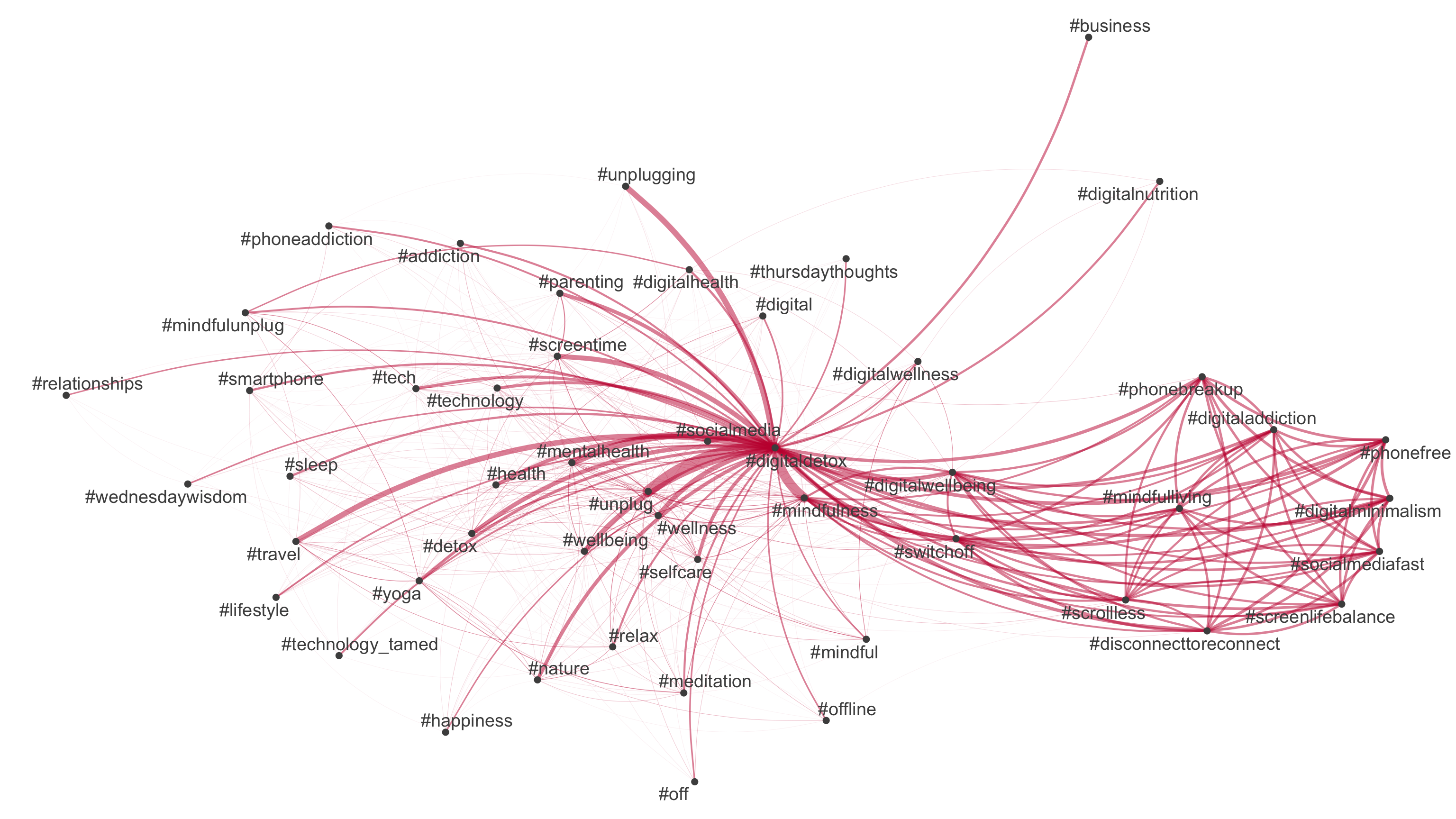
# Extract DFM with only hashtags
quanteda_dfm_hashtags <- quanteda_dfm %>%
  quanteda::dfm_select(pattern = "#*")

# Extract most common hashtags
top50_hashtags_quanteda <- quanteda_dfm_hashtags %>%
  topfeatures(50) %>%
  names()

# Construct feature-occurrence matrix of hashtags
quanteda_dfm_hashtags %>%
  fcm() %>%
  fcm_select(pattern = top50_hashtags_quanteda) %>%
  textplot_network(
    edge_color = "#C50F3C"
) 
Topic modeling
Preparation
Pruning
quanteda_dfm_trim <- quanteda_dfm %>%
  dfm_trim(
    min_docfreq = 0.0001,
    max_docfreq = .099,
    docfreq_type = "prop"
  )

# Convert for stm topic modeling
quanteda_stm <- quanteda_dfm_trim %>%
    convert(to = "stm")
Converting the trimmmed DFM to an stm object will result in an errormessage
Warning message:
In dfm2stm(x, docvars, omit_empty = TRUE) : Dropped 46,670 empty document(s)
This is due to the fact, that some tweets are “empty” or do not match with any feature after the pruning. To successfully match the stm results with the original data, the “empty” tweets need to be dropped. To identify the empty cases, run
# Check if tweet contains feature
empty_docs <- Matrix::rowSums(as(quanteda_dfm_trim, "Matrix")) == 0

# Create vector for empty tweet identification
empty_docs_ids <- quanteda_dfm_trim@docvars$docname[empty_docs]
# Optional: Print indices of empty documents
if (any(empty_docs)) {
cat("Indices of empty documents:", which(empty_docs), "\n")
# Print corresponding docnames
cat("Docnames of empty documents:", quanteda_dfm_trim@docvars$docname[empty_docs], "\n")
}Select model
based on k = 0
# Estimate model
stm_k0 <- stm(
    quanteda_stm$documents,
    quanteda_stm$vocab,
    K = 0,
    max.em.its = 50,
    init.type = "Spectral",
    seed = 42
  )
# Preview
stm_k0A topic model with 72 topics, 46574 documents and a 8268 word dictionary.based on different model diagnostics
# Set up parallel processing using furrr
future::plan(future::multisession()) # use multiple sessions

# Estimate multiple models
stm_exploration <- tibble(k = seq(from = 5, to = 85, by = 5)) %>%
    mutate(mdl = furrr::future_map(k, ~stm::stm(
      documents =  quanteda_stm$documents,
      vocab = quanteda_stm$vocab,
      K = .,
      seed = 42,
      max.em.its = 1000,
      init.type = "Spectral",
      verbose = FALSE),
      .options = furrr::furrr_options(seed = 42))
)stm_exploration$mdl[[1]]
A topic model with 5 topics, 46574 documents and a 8268 word dictionary.
[[2]]
A topic model with 10 topics, 46574 documents and a 8268 word dictionary.
[[3]]
A topic model with 15 topics, 46574 documents and a 8268 word dictionary.
[[4]]
A topic model with 20 topics, 46574 documents and a 8268 word dictionary.
[[5]]
A topic model with 25 topics, 46574 documents and a 8268 word dictionary.
[[6]]
A topic model with 30 topics, 46574 documents and a 8268 word dictionary.
[[7]]
A topic model with 35 topics, 46574 documents and a 8268 word dictionary.
[[8]]
A topic model with 40 topics, 46574 documents and a 8268 word dictionary.
[[9]]
A topic model with 45 topics, 46574 documents and a 8268 word dictionary.
[[10]]
A topic model with 50 topics, 46574 documents and a 8268 word dictionary.
[[11]]
A topic model with 55 topics, 46574 documents and a 8268 word dictionary.
[[12]]
A topic model with 60 topics, 46574 documents and a 8268 word dictionary.
[[13]]
A topic model with 65 topics, 46574 documents and a 8268 word dictionary.
[[14]]
A topic model with 70 topics, 46574 documents and a 8268 word dictionary.
[[15]]
A topic model with 75 topics, 46574 documents and a 8268 word dictionary.
[[16]]
A topic model with 80 topics, 46574 documents and a 8268 word dictionary.
[[17]]
A topic model with 85 topics, 46574 documents and a 8268 word dictionary.Exploration
# Create heldout
heldout <- make.heldout(
  quanteda_stm$documents,
  quanteda_stm$vocab,
  seed = 42)

# Create model diagnostics
stm_results <- stm_exploration %>%
  mutate(exclusivity = map(mdl, exclusivity),
         semantic_coherence = map(mdl, semanticCoherence, quanteda_stm$documents),
         eval_heldout = map(mdl, eval.heldout, heldout$missing),
         residual = map(mdl, checkResiduals, quanteda_stm$documents),
         bound =  map_dbl(mdl, function(x) max(x$convergence$bound)),
         lfact = map_dbl(mdl, function(x) lfactorial(x$settings$dim$K)),
         lbound = bound + lfact,
         iterations = map_dbl(mdl, function(x) length(x$convergence$bound)))
# Preview
stm_results# A tibble: 17 × 10
k mdl exclusivity semantic_coherence eval_heldout residual bound
<dbl> <list> <list> <list> <list> <list> <dbl>
1 5 <STM> <dbl [5]> <dbl [5]> <named list> <named list> -3.25e6
2 10 <STM> <dbl [10]> <dbl [10]> <named list> <named list> -3.21e6
3 15 <STM> <dbl [15]> <dbl [15]> <named list> <named list> -3.17e6
4 20 <STM> <dbl [20]> <dbl [20]> <named list> <named list> -3.12e6
5 25 <STM> <dbl [25]> <dbl [25]> <named list> <named list> -3.09e6
6 30 <STM> <dbl [30]> <dbl [30]> <named list> <named list> -3.09e6
7 35 <STM> <dbl [35]> <dbl [35]> <named list> <named list> -3.08e6
8 40 <STM> <dbl [40]> <dbl [40]> <named list> <named list> -3.07e6
9 45 <STM> <dbl [45]> <dbl [45]> <named list> <named list> -3.07e6
10 50 <STM> <dbl [50]> <dbl [50]> <named list> <named list> -3.06e6
11 55 <STM> <dbl [55]> <dbl [55]> <named list> <named list> -3.05e6
12 60 <STM> <dbl [60]> <dbl [60]> <named list> <named list> -3.05e6
13 65 <STM> <dbl [65]> <dbl [65]> <named list> <named list> -3.05e6
14 70 <STM> <dbl [70]> <dbl [70]> <named list> <named list> -3.07e6
15 75 <STM> <dbl [75]> <dbl [75]> <named list> <named list> -3.06e6
16 80 <STM> <dbl [80]> <dbl [80]> <named list> <named list> -3.03e6
17 85 <STM> <dbl [85]> <dbl [85]> <named list> <named list> -3.06e6
# ℹ 3 more variables: lfact <dbl>, lbound <dbl>, iterations <dbl># Visualize
stm_results %>%
transmute(
k,
`Lower bound` = lbound,
Residuals = map_dbl(residual, "dispersion"),
`Semantic coherence` = map_dbl(semantic_coherence, mean),
`Held-out likelihood` = map_dbl(eval_heldout, "expected.heldout")) %>%
gather(Metric, Value, -k) %>%
ggplot(aes(k, Value, color = Metric)) +
geom_line(size = 1.5, alpha = 0.7, show.legend = FALSE) +
geom_point(size = 3) +
scale_x_continuous(breaks = seq(from = 5, to = 85, by = 5)) +
facet_wrap(~Metric, scales = "free_y") +
labs(x = "K (number of topics)",
y = NULL,
title = "Model diagnostics by number of topics"
) +
theme_pubr() +
# add highlights
geom_vline(aes(xintercept = 5), color = "#00BFC4", alpha = .5) +
geom_vline(aes(xintercept = 10), color = "#C77CFF", alpha = .5) +
geom_vline(aes(xintercept = 40), color = "#C77CFF", alpha = .5) 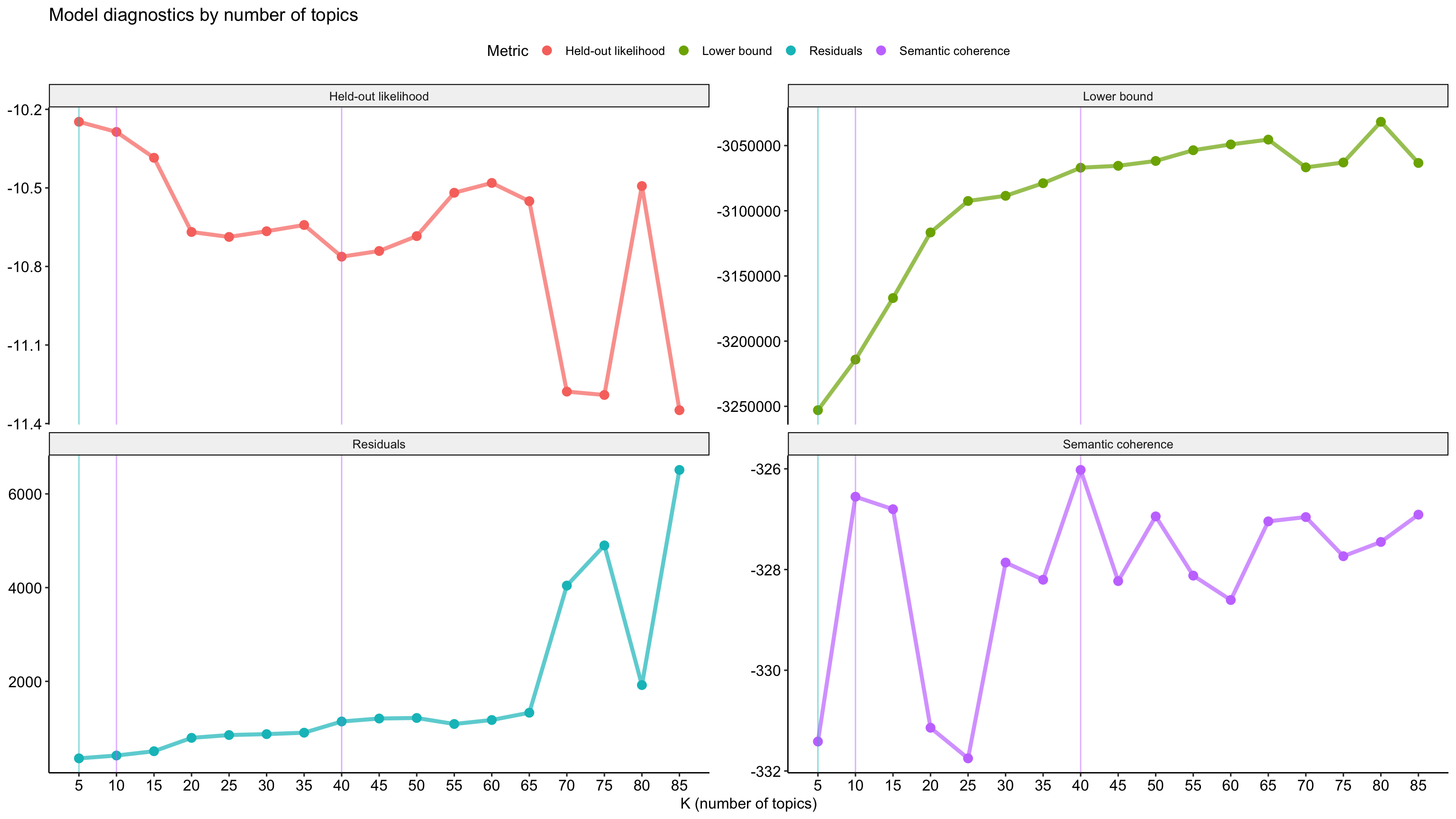
# Models for comparison
models_for_comparison = c(5, 10, 40)

# Create figures
fig_excl <- stm_results %>%
  # Edit data
  select(k, exclusivity, semantic_coherence) %>%
  filter(k %in% models_for_comparison) %>%
  unnest(cols = c(exclusivity, semantic_coherence))  %>%
  mutate(k = as.factor(k)) %>%
  # Build graph
  ggplot(aes(semantic_coherence, exclusivity, color = k)) +
    geom_point(size = 2, alpha = 0.7) +
    labs(
      x = "Semantic coherence",
      y = "Exclusivity"
      # title = "Comparing exclusivity and semantic coherence",
      # subtitle = "Models with fewer topics have higher semantic coherence for more topics, but lower exclusivity"
      ) +
      theme_pubr()

# Create plotly
fig_excl %>% plotly::ggplotly()
Understanding
Select model for further analysis
n_topics <- 10

tpm <- stm_results |>
   filter(k == n_topics) |>
   pull(mdl) %>% .[[1]]
Overview
tpm %>% plot(type = "summary")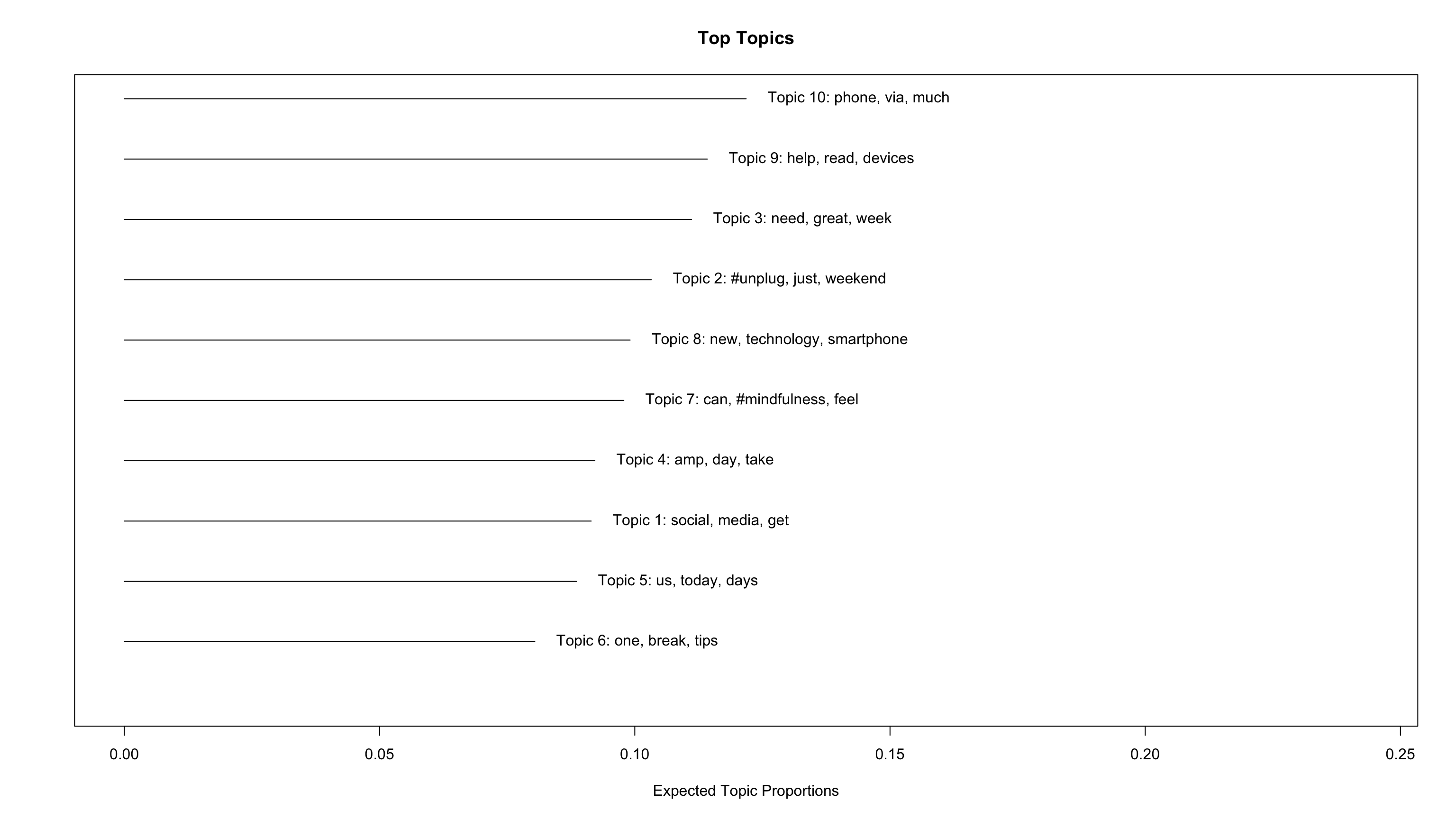
tpm %>% plot(type = "hist")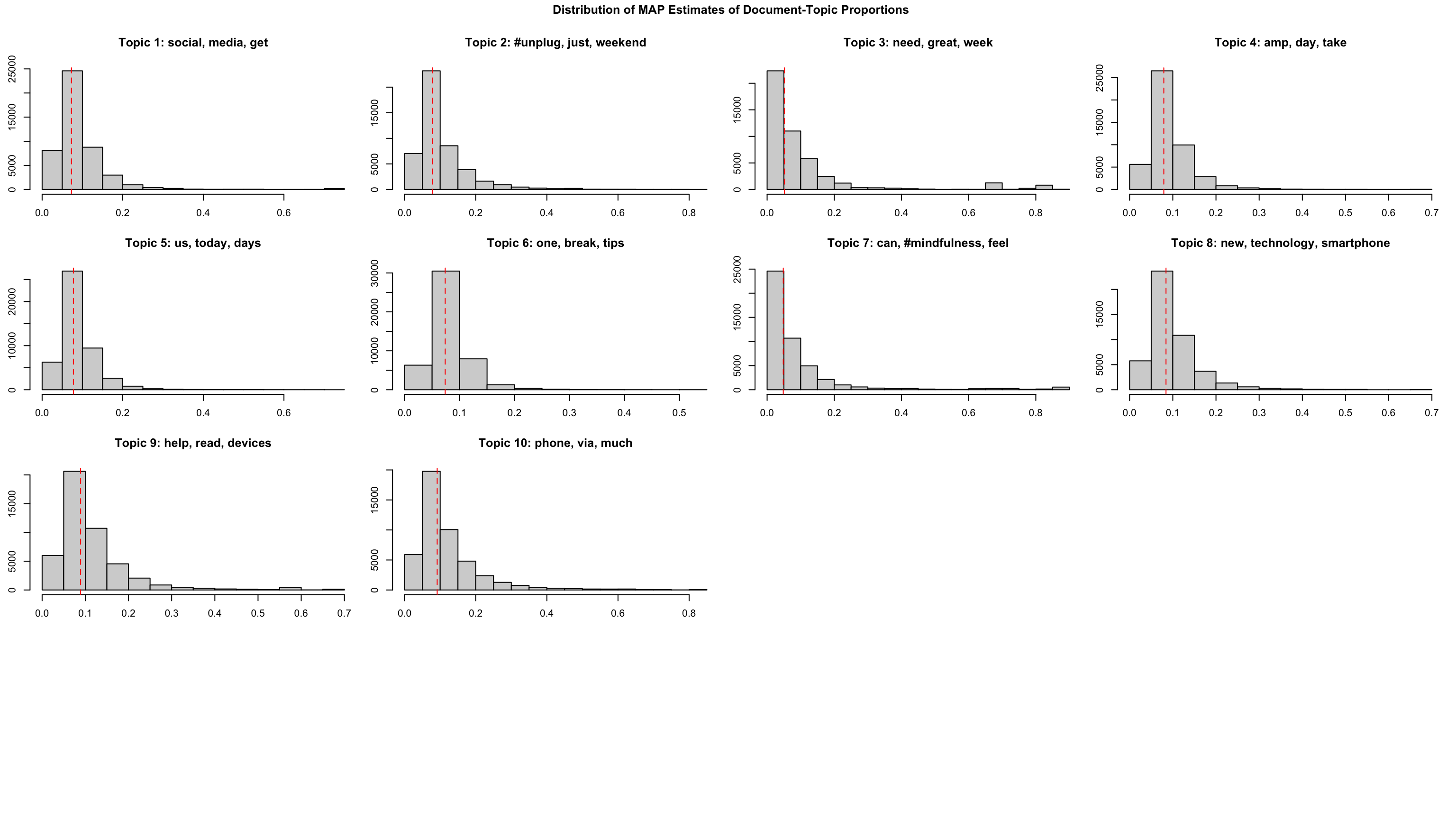
Document/Word-topic relations
# Create data
top_gamma <- tpm %>%
  tidy(matrix = "gamma") %>%
  dplyr::group_by(topic) %>%
  dplyr::summarise(gamma = mean(gamma), .groups = "drop") %>%
  dplyr::arrange(desc(gamma))

top_beta <- tpm %>%
  tidytext::tidy(.) %>%
  dplyr::group_by(topic) %>%
  dplyr::arrange(-beta) %>%
  dplyr::top_n(10, wt = beta) %>%
  dplyr::select(topic, term) %>%
  dplyr::summarise(terms_beta = toString(term), .groups = "drop")

top_topics_terms <- top_beta %>%
  dplyr::left_join(top_gamma, by = "topic") %>%
  dplyr::mutate(
          topic = paste0("Topic ", topic),
          topic = reorder(topic, gamma)
      )

# Preview
top_topics_terms %>%
  mutate(across(gamma, ~round(.,3))) %>%
  dplyr::arrange(-gamma) %>%
gt()| topic | terms_beta | gamma |
|---|---|---|
| Topic 10 | phone, via, much, #screentime, know, check, people, phones, #parenting, online | 0.122 |
| Topic 9 | help, read, devices, use, world, tech, family, taking, kids, sleep | 0.114 |
| Topic 3 | need, great, week, going, listen, #unplugging, discuss, @icphenomenallyu, away, well | 0.111 |
| Topic 2 | #unplug, just, weekend, #travel, unplug, enjoy, #nature, really, join, nature | 0.103 |
| Topic 8 | new, technology, smartphone, retreat, work, addiction, year, health, internet, without | 0.099 |
| Topic 7 | can, #mindfulness, feel, #switchoff, #digitalwellbeing, #wellness, things, #phonefree, #disconnecttoreconnect, #digitalminimalism | 0.098 |
| Topic 4 | amp, day, take, #mentalhealth, go, try, #wellbeing, now, give, every | 0.092 |
| Topic 1 | social, media, get, life, back, like, good, #socialmedia, find, see | 0.091 |
| Topic 5 | us, today, days, next, put, happy, may, facebook, share, hour | 0.089 |
| Topic 6 | one, break, tips, make, screen, love, #technology, free, looking, getting | 0.080 |
Document-topic-relations
# Prepare for merging
topic_gammas <- tpm %>%
  tidy(matrix = "gamma") %>%
  dplyr::group_by(document) %>%
  tidyr::pivot_wider(
    id_cols = document,
    names_from = "topic",
    names_prefix = "gamma_topic_",
    values_from = "gamma")

gammas <- tpm %>%
  tidytext::tidy(matrix = "gamma") %>%
  dplyr::group_by(document) %>%
  dplyr::slice_max(gamma) %>%
  dplyr::mutate(main_topic = ifelse(gamma > 0.5, topic, NA)) %>%
  rename(
    top_topic = topic,
    top_gamma = gamma) %>%
  ungroup() %>%
  left_join(., topic_gammas, by = join_by(document))

# Merge with original data
tweets_detox_topics <- tweets_detox %>%
  filter(!(tweet_id %in% empty_docs_ids)) %>%
  bind_cols(gammas) %>%
  select(-document)

# Preview
tweets_detox_topics
# A tibble: 46,574 × 50
tweet_id user_username text created_at in_reply_to_user_id
<chr> <chr> <chr> <dttm> <chr>
1 5777201122 pblackshaw Put down yo… 2009-11-16 22:03:12 <NA>
2 4814687834 andrewgerrard @Dawn_Wylie… 2009-10-12 18:48:30 18003723
3 4813781509 pblackshaw Is Social M… 2009-10-12 17:55:57 <NA>
4 3351604894 KurtyD Google gear… 2009-08-16 23:20:53 <NA>
5 3350930292 KurtyD Wifi on the… 2009-08-16 22:31:22 <NA>
6 3349372574 KurtyD Adios amigo… 2009-08-16 20:37:03 <NA>
7 2722418665 evelynanne Ok, I'm hea… 2009-07-19 14:31:16 <NA>
8 1959962952 halriley I'm thinkin… 2009-05-29 14:11:36 <NA>
9 1638612063 deconst Interesting… 2009-04-28 13:03:14 <NA>
10 1626172818 deconst Back from #… 2009-04-27 03:55:25 <NA>
# ℹ 46,564 more rows
# ℹ 45 more variables: author_id <chr>, lang <chr>, possibly_sensitive <lgl>,
# conversation_id <chr>, user_created_at <chr>, user_protected <lgl>,
# user_name <chr>, user_verified <lgl>, user_description <chr>,
# user_location <chr>, user_url <chr>, user_profile_image_url <chr>,
# user_pinned_tweet_id <chr>, retweet_count <int>, like_count <int>,
# quote_count <int>, user_tweet_count <int>, user_list_count <int>, …Topic distribution
tweets_detox_topics %>%
  mutate(across(top_topic, as.factor)) %>%
  ggplot(aes(top_topic)) +
  geom_bar() +
  theme_pubr()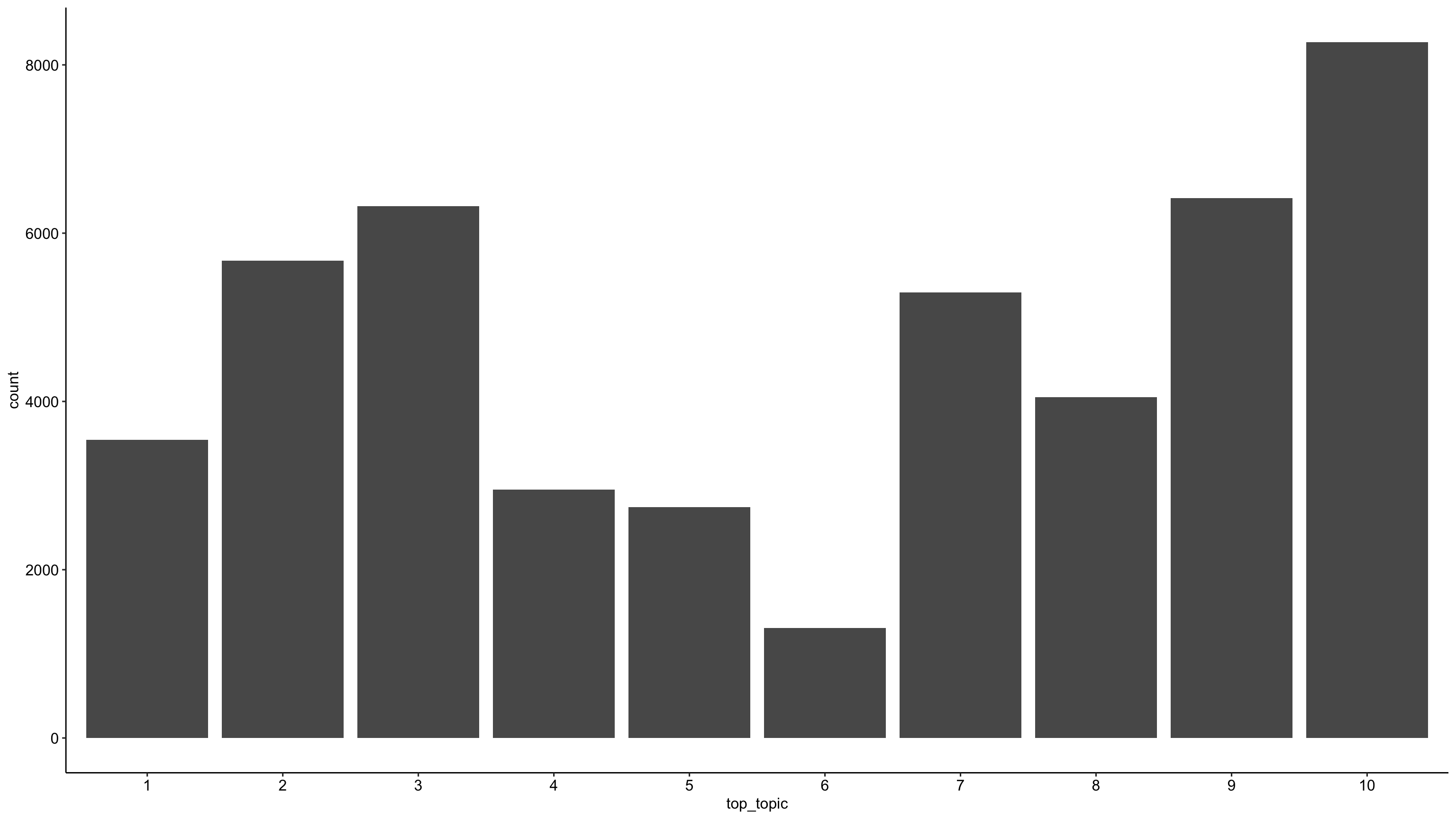
Topic distribution over time
tweets_detox_topics %>%
  mutate(across(top_topic, as.factor)) %>%
  ggplot(aes(year, fill = top_topic)) +
  geom_bar() +
  theme_pubr()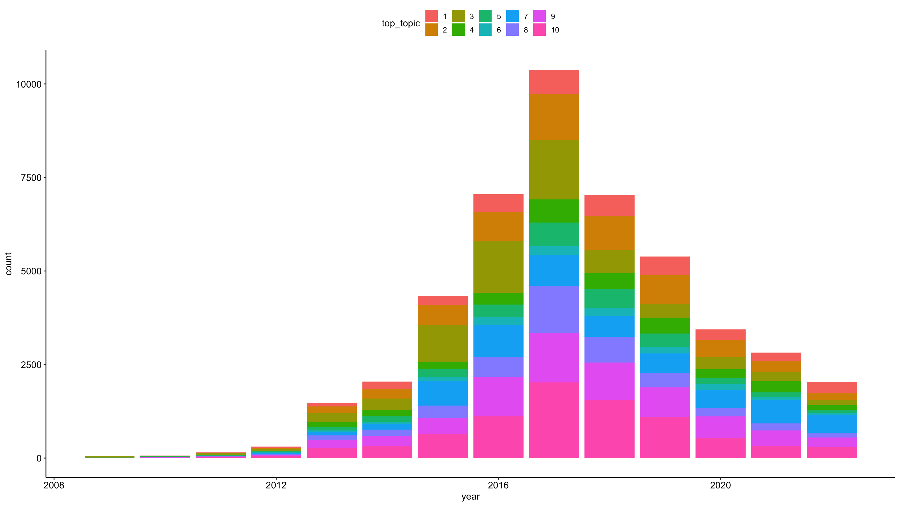
tweets_detox_topics %>%
  mutate(across(top_topic, as.factor)) %>%
  ggplot(aes(year, fill = top_topic)) +
  geom_bar(position = "fill") +
theme_pubr() 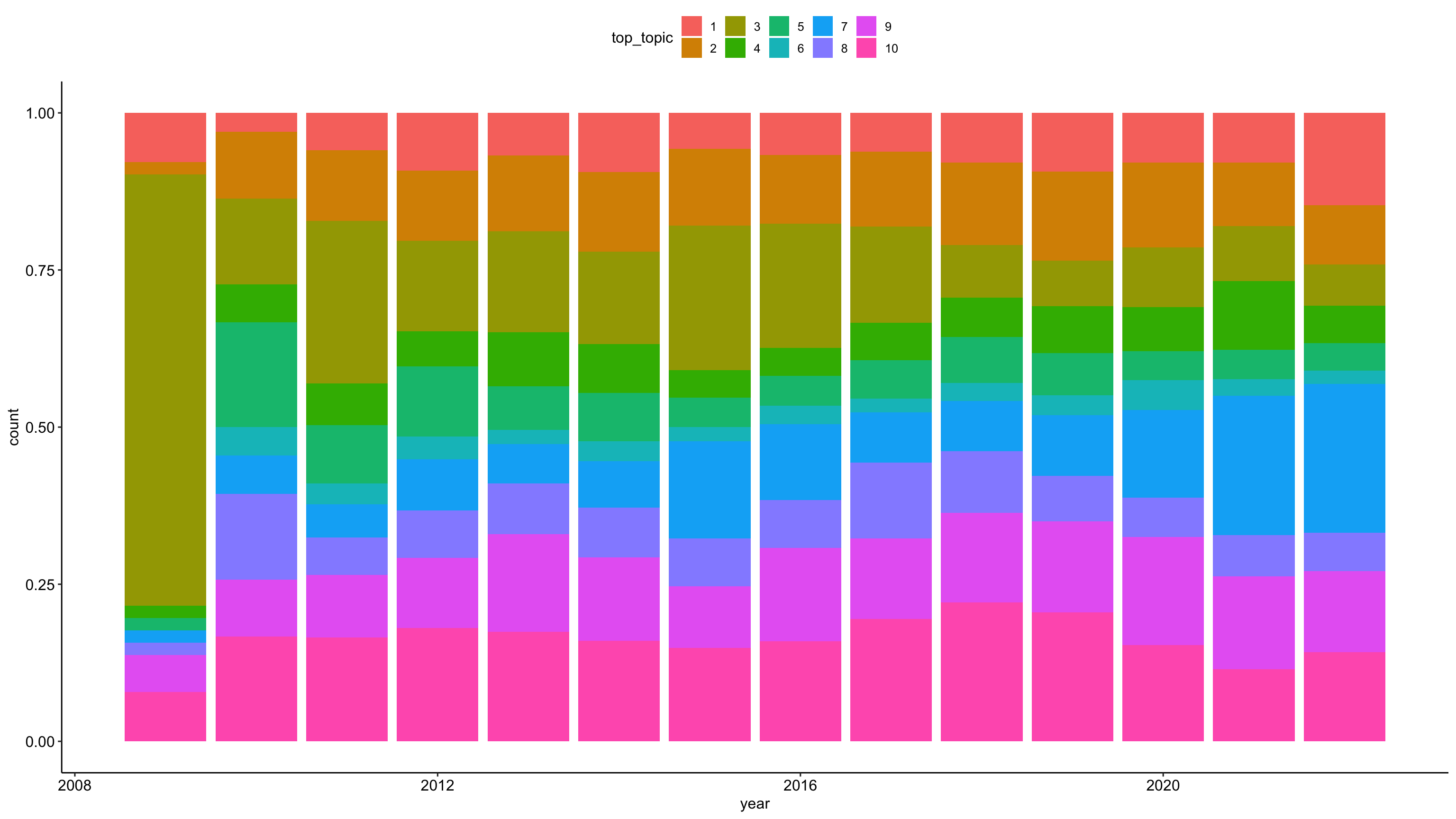
Focus on specific topics
tweets_detox_topics %>%
  filter(top_topic == 10) %>%
  arrange(-top_gamma) %>%
  slice_head(n = 10) %>%
  select(tweet_id, user_username, created_at, text, top_gamma) %>%
gt()| tweet_id | user_username | created_at | text | top_gamma |
|---|---|---|---|---|
| 1496707135794827266 | beckygrantstr | 2022-02-24 04:42:43 | Do you have a blind spot when it comes to what your kids are doing online? #screentime #parenting #digitaldetox Parents Have a Blind Spot When it Comes to Kids and Screens | by Becky Grant | A Parent Is Born | Feb, 2022 | Medium - via @pensignal https://t.co/EcV7yKn4WX | 0.8192142 |
| 1496343978672898048 | beckygrantstr | 2022-02-23 04:39:39 | Do you have a blind spot when it comes to what your kids are doing online? #screentime #parenting #digitaldetox Parents Have a Blind Spot When it Comes to Kids and Screens | by Becky Grant | A Parent Is Born | Feb, 2022 | Medium - via @pensignal https://t.co/o9e6WQIpm5 | 0.8192142 |
| 1495981434665947137 | beckygrantstr | 2022-02-22 04:39:02 | Do you have a blind spot when it comes to what your kids are doing online? #screentime #parenting #digitaldetox Parents Have a Blind Spot When it Comes to Kids and Screens | by Becky Grant | A Parent Is Born | Feb, 2022 | Medium - via @pensignal https://t.co/rQgcPltrMt | 0.8192142 |
| 1499612427503247360 | beckygrantstr | 2022-03-04 05:07:18 | Do you have a blind spot when it comes to what your kids are doing online? #screentime #parenting #digitaldetox Parents Have a Blind Spot When it Comes to Kids and Screens | by Becky Grant | A Parent Is Born | Feb, 2022 | Medium - via @pensignal https://t.co/DQRQlN1iyq | 0.8192142 |
| 1499249315381977089 | beckygrantstr | 2022-03-03 05:04:26 | Do you have a blind spot when it comes to what your kids are doing online? #screentime #parenting #digitaldetox Parents Have a Blind Spot When it Comes to Kids and Screens | by Becky Grant | A Parent Is Born | Feb, 2022 | Medium - via @pensignal https://t.co/L7ly66J2fq | 0.8192142 |
| 1498886117394980865 | beckygrantstr | 2022-03-02 05:01:13 | Do you have a blind spot when it comes to what your kids are doing online? #screentime #parenting #digitaldetox Parents Have a Blind Spot When it Comes to Kids and Screens | by Becky Grant | A Parent Is Born | Feb, 2022 | Medium - via @pensignal https://t.co/uJPIMYY1Id | 0.8192142 |
| 1498522796611321864 | beckygrantstr | 2022-03-01 04:57:30 | Do you have a blind spot when it comes to what your kids are doing online? #screentime #parenting #digitaldetox Parents Have a Blind Spot When it Comes to Kids and Screens | by Becky Grant | A Parent Is Born | Feb, 2022 | Medium - via @pensignal https://t.co/z4Fv2bmeag | 0.8192142 |
| 1498159674008510465 | beckygrantstr | 2022-02-28 04:54:35 | Do you have a blind spot when it comes to what your kids are doing online? #screentime #parenting #digitaldetox Parents Have a Blind Spot When it Comes to Kids and Screens | by Becky Grant | A Parent Is Born | Feb, 2022 | Medium - via @pensignal https://t.co/SdZFAJy6kZ | 0.8192142 |
| 1497796525929472003 | beckygrantstr | 2022-02-27 04:51:34 | Do you have a blind spot when it comes to what your kids are doing online? #screentime #parenting #digitaldetox Parents Have a Blind Spot When it Comes to Kids and Screens | by Becky Grant | A Parent Is Born | Feb, 2022 | Medium - via @pensignal https://t.co/OKLMzwfQUA | 0.8192142 |
| 1497433419512524802 | beckygrantstr | 2022-02-26 04:48:42 | Do you have a blind spot when it comes to what your kids are doing online? #screentime #parenting #digitaldetox Parents Have a Blind Spot When it Comes to Kids and Screens | by Becky Grant | A Parent Is Born | Feb, 2022 | Medium - via @pensignal https://t.co/yTnqhTPV8h | 0.8192142 |
Top Users
tweets_detox_topics %>%
  filter(top_topic == 10) %>%
  count(user_username, sort = TRUE) %>%
  mutate(prop = round(n/sum(n)*100, 2)) %>%
  slice_head(n = 15)
# A tibble: 15 × 3
user_username n prop
<chr> <int> <dbl>
1 TimeToLogOff 2384 28.8
2 punkt 390 4.72
3 petitstvincent 175 2.12
4 tanyagoodin 135 1.63
5 ditox_unplug 111 1.34
6 OurHourOff 99 1.2
7 beckygrantstr 63 0.76
8 CreeEscape 56 0.68
9 ConsciDigital 51 0.62
10 phubboo 50 0.6
11 digitaldetoxing 47 0.57
12 smudgedlippy 40 0.48
13 detox_india 32 0.39
14 winiepuh 27 0.33
15 iamscentered 23 0.28References
Barrie, Christopher, and Justin Ho. 2021. “academictwitteR: An r Package to Access the Twitter Academic Research Product Track V2 API Endpoint.” Journal of Open Source Software 6 (62): 3272. https://doi.org/10.21105/joss.03272.
Nassen, Lise-Marie, Heidi Vandebosch, Karolien Poels, and Kathrin Karsay. 2023. “Opt-Out, Abstain, Unplug. A Systematic Review of the Voluntary Digital Disconnection Literature.” Telematics and Informatics 81 (June): 101980. https://doi.org/10.1016/j.tele.2023.101980.